Beyond Mapping III
|
Map
Analysis book with companion CD-ROM
for hands-on exercises and further reading |
Harvesting an Understanding of GIS Modeling — describes
a prototype model for assessing off-road access to forest areas
Extending Forest Harvesting’s Reach — discusses
a multiplicative weighting method for model extension
A Twelve-step
Program for Recovery from Flaky
Forest Formulations — describes
a spatial model for identifying Landings and Timbersheds
E911 for the
Backcountry — describes
development of an on- and off-road travel-time surface for emergency response
Optimal Path Density isn’t all that
Conceptually Dense — discusses
the use of Optimal Path Density to identify corridors of common access
Extending Emergency
Response Beyond the Lines — discusses
basic model processing and modifications for additional considerations
Comparing
Emergency Response Alternatives — describes
comparison
procedures and route evaluation techniques
Bringing Travel and Terrain
Directions into Line — describes
comparison
procedures and route evaluation techniques
Assessing Wildfire Response (Part 1):
Oneth by Land, Twoeth
by Air — discusses a
spatial model for determining effective helicopter landing zones
Assessing Wildfire Response (Part 2):
Jumping Right into It — describes
map analysis
procedures for determining initial response time for alternative attack modes
Mixing It up in GIS
Modeling’s Kitchen — an
overview of map analysis and GIS modeling considerations
Putting GIS
Modeling Concepts in Their Place — develops
a typology of GIS modeling types and characteristics
A Suitable Framework
for GIS Modeling — describes
a framework for suitability modeling based on a flowchart of model logic
GIS’s Supporting Role
in the Future of Natural Resources — discusses the influence of human dimensions in natural
resources and GIS technology’s role
Note: The processing and figures
discussed in this topic were derived using MapCalcTM
software. See www.innovativegis.com to download a free
MapCalc Learner version with tutorial materials for classroom and self-learning
map analysis concepts and procedures.
<Click here>
right-click to download a printer-friendly version of this topic (.pdf).
(Back to the Table of Contents)
______________________________
Harvesting
an Understanding of GIS Modeling
(GeoWorld, April 2010)
Vast regions of the Rocky
Mountains are under attack by mountain pine beetles and a blanket of brown is
covering many of the hillsides. Dead and
dying trees stretch to the horizon. In
five years there will be just sticks poking up and within twenty years the
forest floor will look like a game of “pick-up sticks” with a new forest poking
through.
It’s an ecological cycle,
but it is both aggravated by and aggravating to many of us who live and play in
the shadows of the mountains. Is there something
we can do to contain the spread and hasten the regenerative cycle? One suggestion is to remove the dead wood to
speed forest health and convert it to useful products to boot.
This appears attractive
but just knowing there are giga-tons of beetle-gnawed
biomass awaiting “wood utilization” solutions isn’t a fully actionable
answer. What products are viable? Where and how much harvesting is appropriate?
These two basic questions
captured the attention of combined graduate project teams at the University of
Denver. A “capstone MBA” team focused on
the business case while a “GIS modeling” team focused on the geographic
considerations. Their joint experience
in identifying, describing and evaluating potential solutions provided an
opportunity to get their heads around a complex issue requiring integration of
spatial and non-spatial analysis, both at a macro state-wide level and a micro
local level. The experience also
provides a springboard for a short Beyond Mapping series on GIS modeling (scar
tissue and all).
Our outside collaborators
(a non-profit organization and a large energy company) narrowed the
investigation to biomass for augmentation of base-load electric energy
generation—first lesson, always heed the client’s interests. This assumption narrows the macro
considerations as haul distances from a plant are critical. Considering mountainous travel, buffering to
a simple geographic distance is insufficient and travel-time zones were recommended—second
lesson, clients love the on-road travel-time concept.
The concept of modeling
off-road access, on the other hand, is a bit harder to appreciate. It was decided that a micro level
“proof-of-concept prototype model” for assessing forest access would be
developed. Figure 1 depicts the map
variables and basic approach taken for a hypothetical demonstration area—third
lesson, never use real data for a prototype model if you want clients to
concentrate on model logic.
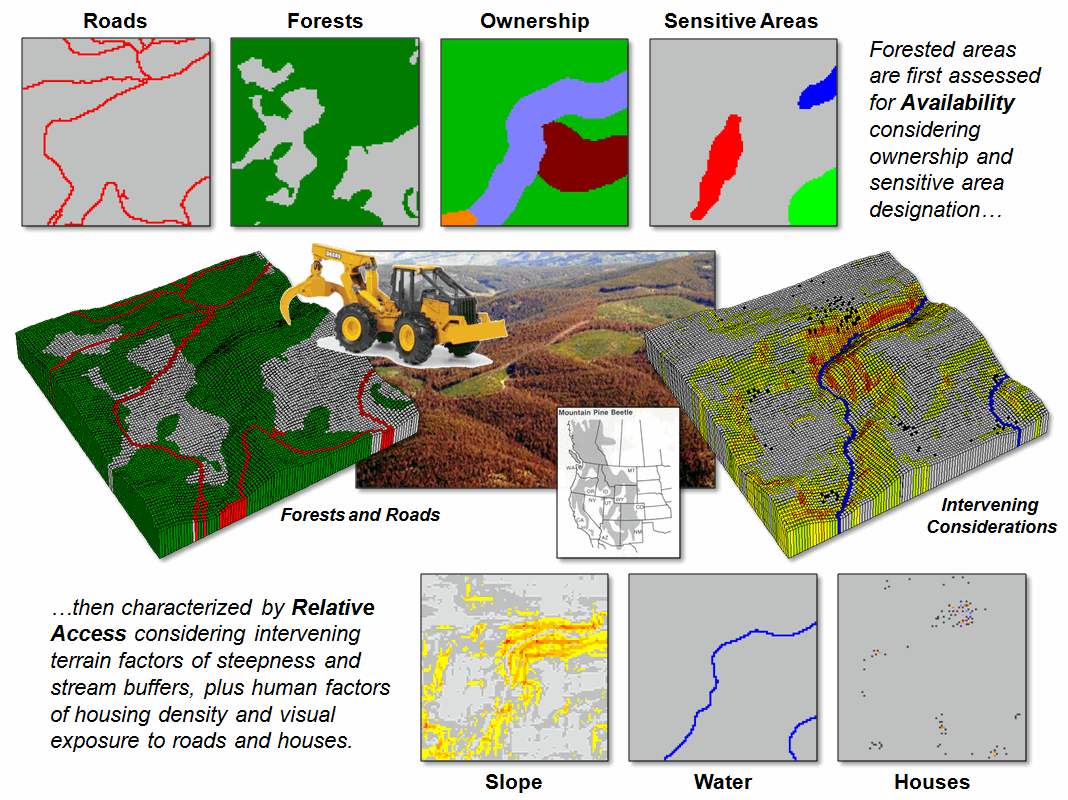
Figure 1. Relative harvesting access is
determined by availability of forest lands as modified by intervening
conditions.
The first phase of the
basic model determines Availability of lands for harvesting
activity. Legal concerns, such as
ownership, stream buffers and sensitive areas must be identified and
unavailable lands removed from further consideration. In addition, physical conditions can become
“absolute barriers,” such as steep slopes beyond the operating range of
equipment. A second phase characterizes
the relative Access of available lands by considering intervening
conditions as “relative barriers,” such as increasing slope in operable areas
increases costs of harvesting.
It is important not to
“over-drive” the purpose of a Prototype Model as a mechanism for demonstrating
a viable approach and stimulating discussion—fourth lesson, “keep it simple
stupid (KISS)” to lock a client’s focus on model approach and logic. Anticipated refinements should be reserved
for a “Further Considerations” section in the presentation describing the
prototype model.
If model refinement
accompanies prototype development, there isn’t a need for a prototype.
But that is the bane of a “waterfall approach” to GIS modeling. You can easily drown by jumping off the edge
at the onset; whereas calmly walking into the pool with your client engages and
involves them, as well as bounds a
manageable first cut of the approach and logic … baby steps with a
client, not a top-down GIS’er solution out of the
box. Fifth lesson—there is a sweet spot along a client’s perception of
a model from a Black box of confusion to Pandora’s box
of terror.
Figure 2. Flowchart of the basic model involves four base maps and ten processing
commands.
Figure 2 contains a
flowchart of model logic for the basic Availability/Access prototype
model. Only four base maps and ten
commands are involved in a demonstrative first cut. A Slope map is used to derive slope impedance
where ranges of steepness are assigned 1 (most preferred)=
0-10%, 2= 10-20%, 4= 20-30% 7 (seven times less preferred)= 30-40% and 0
(unavailable)= >40%. The other maps
of Ownership, Water and Sensitive Areas are used to derive binary maps where 1=
available and 0= unavailable lands. The
final step calculates the acreage of accessible forests within each watershed.
The four calibrated maps
are multiplied for a Discrete Cost Surface that contains a zero for unavailable
lands (any 0 in the map stack sends that location to 0) and the relative
“friction values” based on terrain steepness are preserved for available areas
(1 * 1* 1 * friction value retains that value).
In turn, this map is used to generate the relative access map using a
“Least Cost” approach that will be discussed in next month’s column that “lifts
the hood” on technical considerations (see Author’s note).
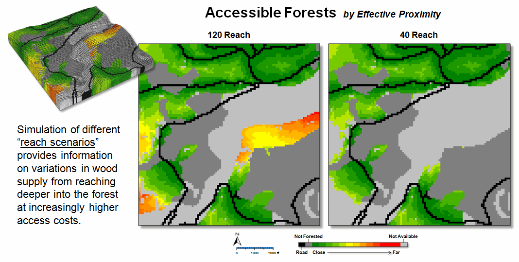
Figure 3. Different effective “reaches” into the accessible forested areas can be
generated to simulate varying budget sensitivities.
Figure 3 provides an
early peek at some of the output generated by the basic Forest Access
model. The left inset shows the relative
access values for all of the available forested areas with warmer tones
indicating a long harvesting reach into the woods; light grey, unavailable and
dark grey, non-forested. A user can
conjure up different “reach” scenarios defining accessible forests as a means
to understand the spatial relationships from grabbing just the “low hanging
economic fruit (…err, I mean wood)” that is easily accessed (right inset), to
increasingly aggressive plunges deeper into the woods at increasingly higher
access costs.
Also, consideration of
human concerns, such as housing density and visual exposure, might affect a
practical assessment of the access reach.
Finally, locating suitable staging areas (termed “Landings”) for wood
collection and the delineation of the forest areas they serve (termed
“Timbersheds”) provide even more fodder for next couple of columns.
_____________________________
Author’s Note: For a discussion on “Calculating Effective Distance and Connectivity” see the online
book, Beyond Mapping III, Topic
25, posted at www.innovativegis.com/basis/MapAnalysis/.
Extending Forest Harvesting’s
Reach
(GeoWorld, May 2010)
The previous section
described a basic spatial model for determining relative harvesting
availability and accessibility of beetle-killed forests for harvesting. The prototype model was developed by
“capstone MBA” and “GIS modeling” graduate teams at the University of
Denver. A non-profit organization and a
large energy company served as outside collaborators and narrowed the focus to
the extraction of biomass for base-load electrical energy generation.
State-wide analysis
involving on-road travel was proposed for assessing hauling distances of wood
chips to power plants where the resource would be further refined and mixed
with coal. Adjusting for mountainous
travel along the road network, some beetle-kill areas simply are too far from a
plant for consideration.
Local level analysis
involving off-road harvesting is considerably more complex. In summary, this processing determines the relative
accessibility from the landings into the forest considering a variety of
terrain, ownership and environmental considerations. Adjusting for off-road access, some
beetle-kill areas are unavailable or effectively too far from roads for
harvesting.
The Basic Access Model
outlined in the top portion of figure 1 demonstrates the types of factors that
can be considered in assessing off-road access.
The processing first identifies absolute barriers to harvesting based
on ownership, environmentally sensitive areas, water buffers and terrain that
is too steep for equipment to operate.
These factors are represented as binary map layers with 1= available and
0= unavailable for harvesting activity.
Relative barriers to forest access are rated from 1= most preferred
to 9= least preferred. In the prototype
model, slopes within the harvesting equipment operating range are used to
demonstrate relative barriers with increasingly steeper slopes becoming less
and less desirable. Multiplying the
stack of map layers identifying absolute and relative barriers results in an
overall preference surface for harvesting with values from 0 (no-go), to 1
(best) through 9 (worst). The final step
uses grid-based effective distance techniques to determine the relative
accessibility of available forested areas from roads (see author’s note).
As an extension to the
basic model, human concerns for minimizing visual exposure and housing density
are outlined in the lower portion of figure 1.
The procedure first derives a visual exposure density surface
identifying the number of times each location is seen from houses and roads and
then calibrates the exposure from .5 (low exposure) through 1.0 (high
exposure). Similarly, a housing density
surface identifying the number of houses within a half mile radius was
calibrated from .5 (low density) to 1.0 (high density). The two adjusted maps are averaged for an
overall weighting factor for each map location.
When the multiplicative
weight is applied to the preference map stack, it improves (lowers) preference
ratings in areas with low visual exposure and housing density, while retaining
the basic ratings in areas of high visual exposure and housing density. The effect on the model is to favor reaching
farther into available forested areas in locations that are less
contentious.
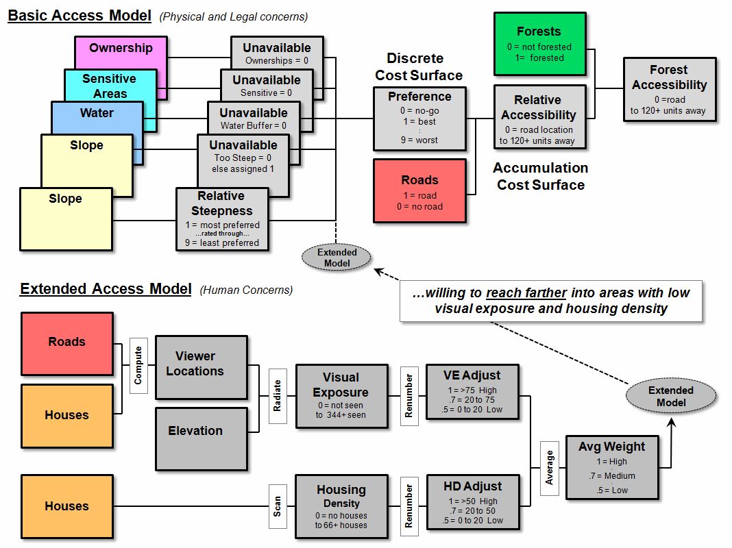
Figure 1. The Extended Access Model
develops a multiplicative weighting factor based on housing density and visual
exposure of potential harvesting areas.
Figure 2 compares the
results with the left side of the figure tracking the results of Basic Model
and the right side tracking the results of the Extended Model that favors
harvesting in areas of low human impact.
The effective distance to the farthest available forest location is
reduced by a third from 116 to 76. The
3D plots on the bottom of the figure (insets c and d) depict the results as
bowl-shaped accumulation surfaces with the lowest value of 0 “cells away” from
the road in the lower center portion of the project area. Note the considerable easing (lower values;
flattening of the surface) of the relative proximity at the circled remote
location.
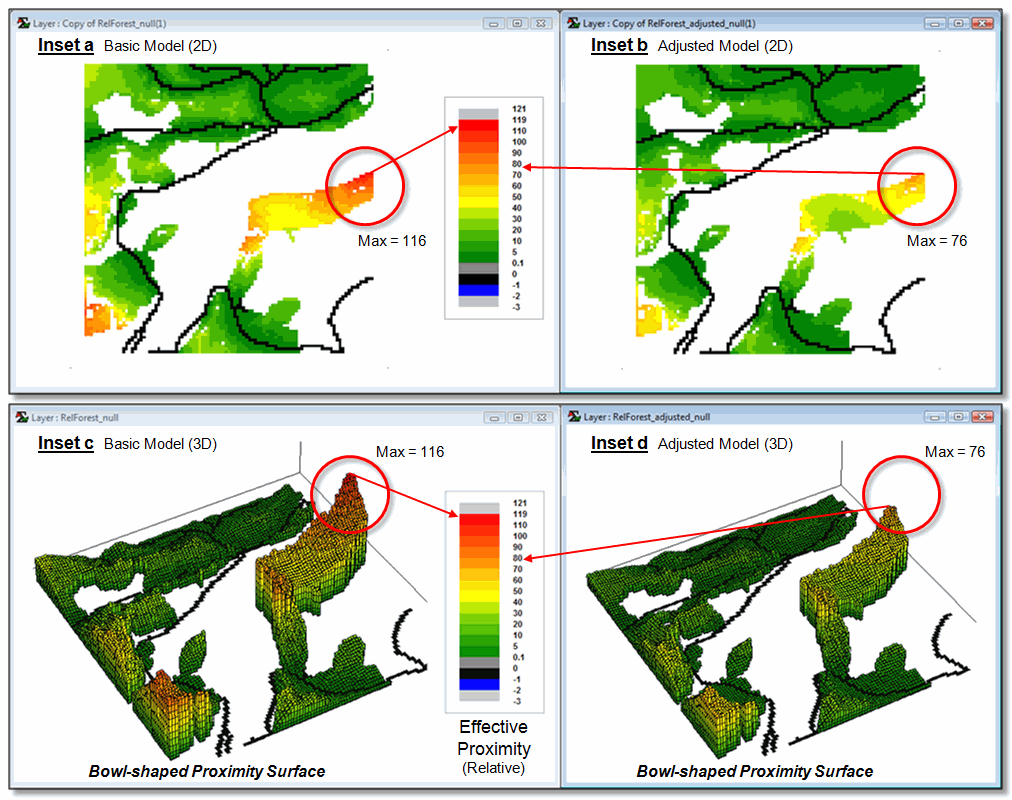
Figure 2. Comparison of Basic and Extended model results.
Figure 3 illustrates a
couple of techniques for summarizing related map information using a binary map
of accessible forest areas. A
region-wide (zonal) overlay operation can be used to “count” the total number
of acres of accessible forest in each of the three watersheds (e.g., 374 aces
of accessible forest in Watershed 3).
Also, by simply multiplying the binary map times the vegetation map
identifies the vegetation type and area for all of the accessible forest
locations (e.g., 964 acres of accessible Lodgepole pine).
The ability to repackage
all beetle-kill areas into those meeting harvesting availability and access
requirements is critical. Just knowing
that there are giga-tons of biomass out there isn’t
sufficient until they are mapped within a comprehensive decision-making
context. The next section explores
procedures for determining the best set of staging areas, termed “landings,”
and the characterization of the potential wood chip supply within each of their
corresponding “timbersheds.”
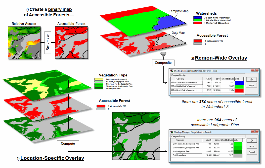
Figure 3. D. Summarizing accessible forest areas by watersheds and vegetation
type.
_____________________________
Author’s Note: For a discussion on “Calculating Effective Distance and Connectivity” see the online
book, Beyond Mapping III, Topic 25,
posted at www.innovativegis.com/basis/MapAnalysis/.
A Twelve-step Program for Recovery from Flaky Forest Formulations
(GeoWorld, June 2010)
The last two sections
described a basic spatial model for determining forest availability and access
considering physical and legal factors that, in turn, was extended to include
human concerns of housing density and visual exposure to harvesting
activity. This column builds on those
procedures for a further formulated model that 1) identifies the best set of
staging areas for wood collection, termed “Landings” and 2) delineates
the harvest areas optimally connected to each landing, termed “Timbersheds.”
The model involves
logical sequencing of twelve standard map analysis steps that are described
using MapCalc commands that are easily translated into other grid-based
software systems (see author’s note).
The top portion of figure 1 uses the five “binary maps” created in the
basic model to generate a map of potential landing areas. The maps are calibrated as 1 = available and
0 = not available for harvesting, and when multiplied together (1. Compute)
results in 1 being assigned to all roads locations passing through available
forest areas— 1*1*1*1*1= 1; if a zero appears in any map layers it results in a
0 value (not a road in an available forest area).
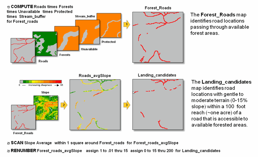
Figure 1. Identifying candidate Landing Sites that are
along forested roads
in gently sloped areas (steps 1-3).
The lower portion of
figure 1 depicts using a neighborhood/focal summary operation (2. Scan)
to calculate the average slope within a 100-foot reach of the each forested
road cell. The third step (3.
Renumber) eliminates potential landing areas that that are in areas with
fairly steep surrounding terrain (> 15% average slope). The result is removal of over two thirds of
the total number of road locations.
Figure 2 shows processing
steps 4 through 9 used to locate the best landing sites. In step 4, the Discrete Cost map indicating
the relative ease of equipment operation created in the basic model is masked (4.
Compute) to constrain harvesting activity to just the forested areas. The Accumulated Proximity from roads is calculated
(5. Spread) resulting in an effective distance value for each forest
location that respects the intervening terrain conditions from forested
roads.
The optimal path from
each forest location to its nearest road location is determined and the set of
paths are counted for each map location (6. Drain) resulting in an
Optimal Path Density surface. The insets
in the upper-right portion of figure 2 shows 2D and 3D displays of this
less-than-intuitive surface. Note the
yellow and red tones where many forest locations are optimally accessed—with
one road location in the southern portion of the project area servicing 785
forested locations. The long red path
leading to this location is analogous to a primary road where more and more
collector streets join the overall best route.
Figure 2. Locating the best Landing
Sites based on optimal path density (steps 4-9).
The summary statistics,
along with expert judgment is used to identify an appropriate final set of
landing sites that is suitably dispersed throughout the project area (10.
Renumber) as depicted in the upper portion of figure 3. These final locations for Landings are
used to derive new effective distance values for each forest location
considering intervening terrain conditions (11. Spread) in a manner
similar to step 5. Finally, expert
judgment is used to limit the reach in each of the Timbersheds to a manageable
distance (12. Renumber).
The lower portion of
figure 2 shows the steps for isolating the best landing sites. The highest levels of optimal path density
are isolated (7. Renumber) and then masked to identify the forested road
locations with the highest optimal path density (8. Compute). In turn these locations are assigned a unique
ID value (9. Clump) and summary statistics on each of the “best”
potential landing sites are generated.
Figure 3. Identifying and
characterizing the Timbersheds of the best Landing Sites (steps 10-12).
To put the spatial analysis
into a decision context, a “thumbnail” estimate of the wood chip resource for Timbershed #15 is 164ac * 40T/ac = 6560 tons. At $15 to $30 per ton this converts to 6560T
* $22.50 = $147,600. From another
perspective, assuming 6000 to 8000 btu
per pound of woodchips the energy stored in the biomass translates to 6560T *
2000lb/T * 7000btu/lb = 91,840,000,000 btu. At 3412 btu per kilowatt hour this converts to
91,840,000,000btu / 3412btu/kWh = nearly 27 million kilowatt hours …whew!
Any way you look at it
there is a lot of energy locked up in the giga-tons
of beetle-gnawed biomass blanketing the Rockies. GIS modeling of its availability and access
is but one of several critical steps needed in determining the economic,
environmental and social viability of a “wood utilization” solution.
_____________________________
Author’s Note: See http://www.innovativegis.com/basis/MapCalc/MCcross_ref.htm
for cross-reference of MapCalc commands to other software systems. An animated
PowerPoint slide set of this 3-part Beyond Mapping series on “Assessing and
Characterizing Relative Forest Access” and materials for a “hands-on” exercise are posted at www.innovativegis.com/basis/MapAnalysis/Topic29/ForestAccess.htm.
E911 for the Backcountry
(GeoWorld, July 2010)
One of the most important
applications of geotechnology has been Enhanced 911 (E911) location technology
that enables emergency services to receive the geographic position of a mobile
phone. The geographic position is
automatically geo-coded to a street address and routing software is used to
identify an optimal path for emergency response. But what happens if the call that “I’ve
fallen and can’t get up” comes from a backcountry location miles from a
road? The closest road location “as the
crow flies” is rarely the quickest route in mountainous terrain.
A continuous space
solution is a bit more complex than traditional network analysis as the
relative and absolute barriers for emergency response are scattered about the
landscape. In addition, the intervening
conditions affect modes of travel differently.
For example, an emergency response vehicle can move rapidly along the
backcountry roads, and then all terrain vehicles (ATV) can be employed off the
roads. But ATVs cannot operate under
extremely steep and rugged conditions where hiking becomes necessary.
Figure 1. On-road
emergency response travel-time.
The left side of figure 1
illustrates the on-road portion of a travel-time (TT) surface from headquarters
along secondary backcountry roads. The
grid-based solution uses friction values for each grid cell in a manner
analogous to road segment vectors in network analysis. The difference being that each grid cell is
calibrated for the time it takes to cross it (0.10 minute in this simplified
example).
The result is an estimate
of the travel-time to reach any road location.
Note that the on-road surface forms a rollercoaster shape with the
lowest point at the headquarters (TT = 0 minutes away) and progressively
increases to the farthest away location (TT = 26.5 minutes). If there are two or more headquarters, there
would be multiple “bottoms” and the surface would form ridges at the
equidistance locations in terms of travel-time—each road location assigned a
value indicating time to reach it from the closest headquarters.
The lower-right portion
of figure 1 shows the calibrations for on-road travel by truck and off-road
travel by ATV and hiking as a function of terrain steepness and recognition of
rivers as absolute barriers to surface travel.
The programming trick at this point is to use the accumulated on-road
travel-time for each road location as the starting TT for continued movement
off-road. For example, the off-road locations around the farthest away road location starts
“counting” at
26.5, thereby carrying
forward the on-road travel time to get to off-road locations. As the algorithm proceeds it notes the on- and
off-road travel-time to each ATV accessible location and retains the minimum
time (shortest TT).
Figure 2. On-road plus off-road travel-time
using ATV under operable terrain conditions.
Figure 2 identifies the
shortest combined on- and off-road travel-times. Note that the emergency response solution
forms a bowl-like surface with the headquarters as the lowest point and the
road proximities forming “valleys” of quick access. The sides of the valleys indicate ATV
off-road travel with steeper rises for areas of steeper terrain slopes (slower
movement; higher TT accumulation). The
farthest away location accessible by truck and then ATV is 52.1 minutes.
The grey areas in the
figure indicate locations that are too steep for ATV travel, particularly
apparent in the steep canyon area (lower left insert with warmer tones of Slope
draped over the Elevation surface). The
sharp “escarpment-like” feature in the center of the response surface is caused
by the absolute barrier effect of the river—shorter/easier easier access from
roads west of the river.
Figure 3 completes the
emergency response surface by accounting for hiking time from where the wave
front of the accumulated travel-time by truck and ATV stopped. Note the very steep rise in the surface (blue
tones) resulting from the slow movement in the rugged and steep slopes of the
canyon area. The farthest away location
accessible by truck, then ATV and hiking is estimated at 96.0 minutes.
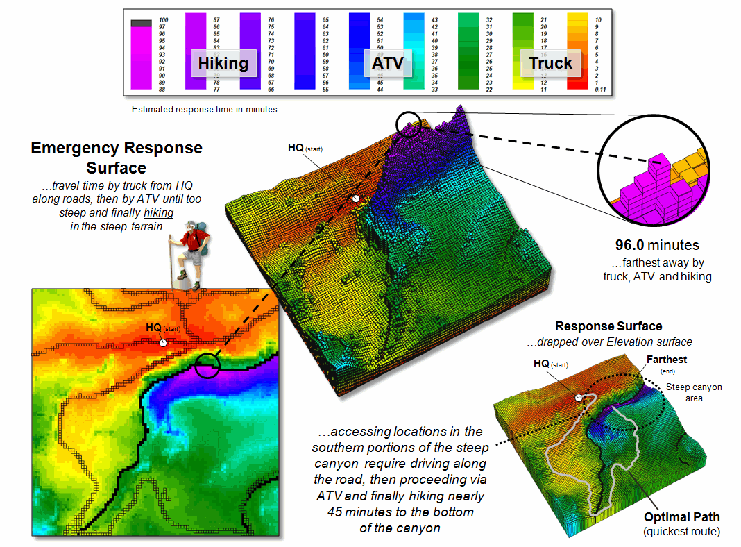
Figure 3. On-road
plus off-road travel-time by ATV and then hiking under extreme terrain
conditions.
The lower-left insert
shows the emergency response values draped over the Elevation surface. Note that the least accessible areas occur on
the southern side of the steep canyon.
The optimal (quickest) path from headquarters to the farthest location
is indicated—that is within the assumptions and calibration of the model.
Later in this topic we
will investigate some alternative scenarios, such as constructing a suspension
bridge at the head of the canyon and identifying helicopter landing areas that
could be used. However the next two
sections investigate travel/terrain interaction and optimal path density to
identify access corridors.
The bottom line of all
this discussion is that GIS modeling can extend emergency response planning
“beyond the lines” of a fixed road network—an important spatial reasoning point
for GIS’ers and non-GIS’ing resource managers alike.
_____________________________
Author’s Note: See www.innovativegis.com/basis/MapAnalysis/Topic29/EmergencyResponse.htm
for an animated slide set illustrating the incremental propagation of the
travel-time wave front considering on- and off-road travel and materials for a
“hands-on” exercise in deriving continuous space emergency response surfaces.
Optimal
Path Density is not all that Dense (Conceptually)
(GeoWorld, January 2013)
The previous section
addressed “Backcountry 911” that considers both on- and off-road travel for
emergency response. Recall that the
approach uses a stepped-accumulation cost surface to estimate travel-time
by truck, then all-terrain vehicle (ATV) and finally hiking into areas too
steep for ATVs.
The result is a map
surface (formally termed an Accumulation Surface) that identifies
the minimum travel-time to reach all accessible locations within a project
area. It is created by employing the
“splash algorithm” to simulate movement in an analogous manner to the
concentric wave pattern propagating out from a pebble tossed into a still pond. If the conditions are the same, the effect is
directly comparable to the uniform set of ripples.
However as the wavefront
encounters varying barriers to movement, the concentric rings are distorted as
they bend and wiggle around the barriers to locate the shortest effective
path. The conditions at each grid location
are evaluated to determine whether movement is totally restricted (absolute
barriers) or, if not, the relative difficulty of the movement (relative
barrier). The end result is a map
surface identifying the “shortest but not necessarily straight line” distance
from the starting location to all other locations in a project area.
The emergency response
surface shown in figure 1 identifies the minimum travel-time via a combination
of truck, ATV and hiking from headquarters (HQ) to all other locations. Travel-time increases with each wavefront
step as a function of the relative difficulty of movement that ultimately
creates a warped bowl-like surface with the starting location at the bottom
(HQ= 0.0 minutes away). The blue tones
identify locations of very slow hiking conditions that result in the “mountain”
of increasing travel-time to the farthest away location (Emergency Location #1=
96.0 minutes away).
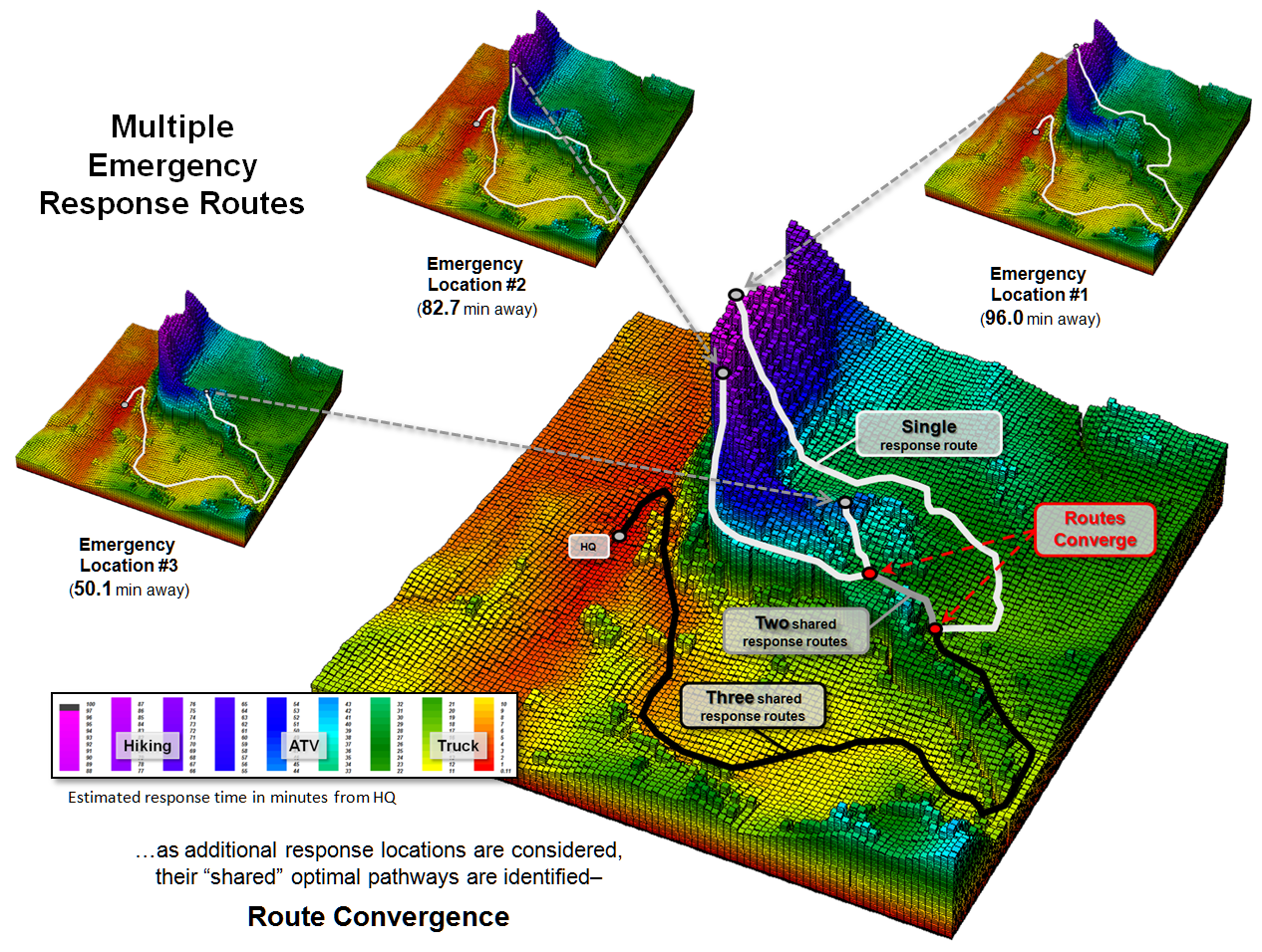
Figure 1. Multiple optimal paths
tend to converge to take advantage of “common access” routes over the
travel-time surface.
The quickest route is
rarely a straight line a crow might fly, but bends and turns depending on the intervening
conditions and how they affect travel.
The Optimal Path (minimum accumulated travel-time route)
from any location is identified as “the steepest downhill path over the
accumulated travel-time surface.”
This pathway retraces the route that the wavefront took as it moved away
from the starting location while minimizing travel-time at each step.
The small plots in the
outer portion of Figure 1 identify the individual optimal paths from three
emergency locations. The larger center
plot combines the three routes to identify their convergence to shared
pathways— grey= two paths and black= all three paths.
The left side of figure 2
simulates responding to all accessible locations in the project area. The result is an “Optimal Path Density”
surface that “counts the number of optimal paths passing through each map
location.” This surface identifies
major confluence areas analogous to water running off a landscape and
channeling into gullies of easiest flow. The light-colored areas
represent travel-time “ridges” that contain no or very few optimal paths. The emergency response “gullies” shown as
darker tones represent off-road response corridors that service large portions
of the backcountry.
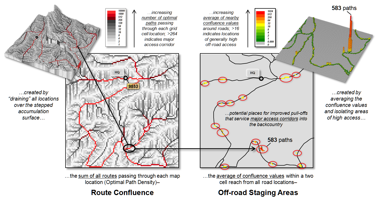
Figure 2. The sum of all optimal
paths passing through a location indicates its relative rating as a “corridor
of common access” for emergency response.
These “corridors of
common access” are depicted as increasingly darker tones that switch to red
for locations servicing more than 256 potential emergency response
locations. Note that 9,853 locations of
the 10,000 locations in the project area “drain” into the headquarters location
(the difference is the non-accessible flowing water locations).
This is powerful
strategic planning information, as well as tactical response routing for
individual emergencies (backcountry 911 routing). For example, knowing where the major access
corridors intersect the road network can be used to identify candidate
locations for staging areas. The right
side of figure 2 identifies fifteen areas with high off-road access that
exceeds an average of sixteen optimal routes within a 1-cell reach from the
road. These “jumping off” points to the
major response corridors might be upgraded to include signage for volunteer
staging areas and improved roadside grading for emergency vehicle parking.
In many ways, GIS
technology is “more different, than it is similar” to traditional mapping and
geo-query. It moves mapping beyond
descriptions of the precise placement of physical features to prescriptions of
new possibilities and perspectives of our geographic surroundings— an Optimal
Path Density surface is but one of many innovative procedures in the new map
analysis toolbox.
_____________________________
Author’s
Note: a free-use poster
and short papers on Backcountry Emergency Response are posted at www.innovativegis.com/basis/Papers/Other/BackcountryER_poster/.
Extending Emergency Response Beyond the Lines
(GeoWorld, August 2010)
The previous section
described a basic GIS model for backcountry emergency response considering both
on- and off-road travel. The process
used grid-based map analysis techniques that consider the spatial arrangement
of absolute barriers (not passable) and relative barriers (passable with
varying ease) that impede emergency response throughout continuous geographic
space.
While the processing
approach is conceptually similar to Network Analysis, movement is not constrained
to a linear network of roads represented as a series of irregular line segments
but can consider travel throughout geographic space represented as a set of
uniform grid cells. The model assumes
that the response team first travels by truck along existing roads, then
off-loads their all-terrain vehicles (ATV) for travel away from the roads until
open water or steep slopes are encountered.
From there the team must proceed on foot. The result of the model is a travel-time map
surface with an estimated minimum response time assigned to each map location
in a project area.
Last section’s discussion
described the key conceptual considerations and results of the three stages of
backcountry emergency response model—truck, ATV and hiking movement. The most notable points were that movement
proceeds as ever increasing waves emanating from a staring location that are
guided by absolute/relative barriers and
results in a continuous travel-time map (bowl-like 3D surface).
Figure 1 outlines the
processing as a flowchart. Boxes
represent map layers and lines represent analysis tools (MapCalc commands are
indicated). The flowchart is organized
with columns characterizing “analysis levels” proceeding from Base maps
(existing data), to Derived maps, to Interpreted maps,
to Modeled map solutions. The
progression reflects a gradient of abstraction from “fact-based” (physical)
characterization of the landscape involving Base and Derived maps, through
increasingly more “judgment-based” (conceptual) characterizations involving
Interpreted and Modeled maps expressing spatial relationships within the
context of a problem.
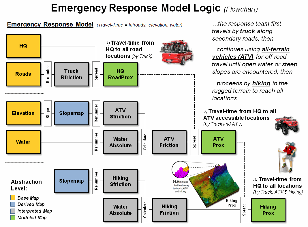
Figure 1. Flowchart
of map analysis processing to establish emergency response time to any location
within a project area.
The row groupings
represent “criteria considerations” used in solving a spatial problem. In this case, the processing first considers
truck travel along the roads then extends the movement off-road by ATV travel
and finally hiking into the areas that are inaccessible by ATV. The off-road movement is guided by open water
(absolute barrier for both ATV and hiking) and terrain steepness (relative
barrier for both ATV and hiking and absolute barrier for ATV in very steep
slopes).
Figure 2 identifies
modifications to the model considering construction of new ATV and hiking
trails and a helipad. The left side of
the figure updates the ATV and hiking “friction” maps with lower travel-time
values for the trails over the unimproved off-road travel impedances. The hiking trail includes a foot bridge at
the head of the canyon that crosses the river.
The revised friction values (ATV trail = 0.15 minutes; hiking trail =
0.5 minutes) directly replace the old values using a single command and the
model is re-executed.
In the case of the new
helipad (right side of the figure) the hiking submodel
is used but with a new starting location that assumes an 18 minute scramble/flight
time to reach the location.
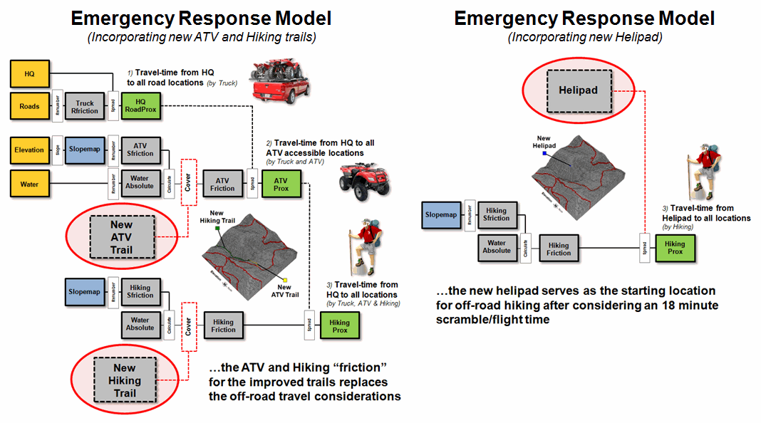
Figure 2. Extended response models
for new trails (left) and helipad (right).
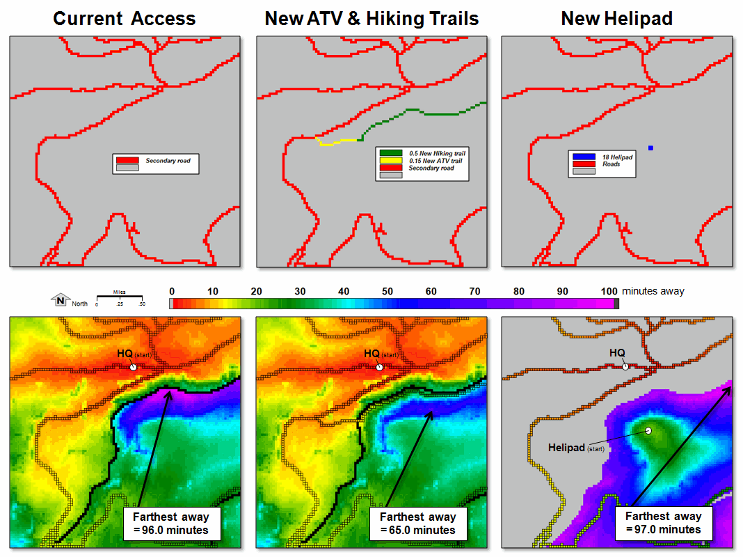
Figure 3. Emergency response
surfaces for the current situation, additional trails and helipad.
The bottom portion of figure
3 shows the three emergency response surfaces.
Visual inspection shows considerable differences in the estimated
response time for the area east of the river.
Current access requires
truck travel across the bridge over the river in the extreme SW portion of the
project area. Construction of the new
trails provides quick ATV access to the foot bridge then easy hiking on the
improved trail along the eastern edge of the river for faster response times on
the east side of the canyon (light blue).
Construction of the new helipad greatly improves response time for the
upper portions of the east side of the canyon.
The next section’s
discussion will focus on quantifying the changes in response time and
developing routing solutions that indicate the type of travel (truck, ATV,
hiking, helicopter) for segments along the optimal path to any location.
_____________________________
Comparing Emergency Response Alternatives
(GeoWorld, September 2010)
The last couple of
sections described a simplified backcountry emergency response model
considering both on- and off-road travel and then extended the discussion by
simulating two alternative planning scenarios—the introduction of a new
ATV/Hiking trail and a Helipad. The
conceptual framework, procedures and considerations in developing the
alternative scenarios were the focus.
This section’s focus is on comparison procedures and route evaluation
techniques.
The left side of figure 1
depicts the minimum expected travel-time from headquarters to all locations
within a project area under current conditions.
The river in the center (black) acts as an absolute barrier that forces
all travel to the southeastern portion across a bridge in the extreme southwest. This makes the farthest away location more
than an hour and a half from the headquarters, although it is less than half a
mile away “as the crow flies.”
The inset in the center
of the figure locates a proposed new ATV/Hiking trail. The first segment of from the road to the
river enables ATV travel. A light
suspension bridge crosses the river to provide hiking access to an improved
trail along the southern side of the canyon.
While the trail is
justified primarily for increasing recreation potential within the canyon, it
has considerable impact on emergency response in the canyon. Note the introduction of the green and light
blue tones along the river that indicate response times of about half an hour
as compared to more than an hour and a half (purple) currently required.
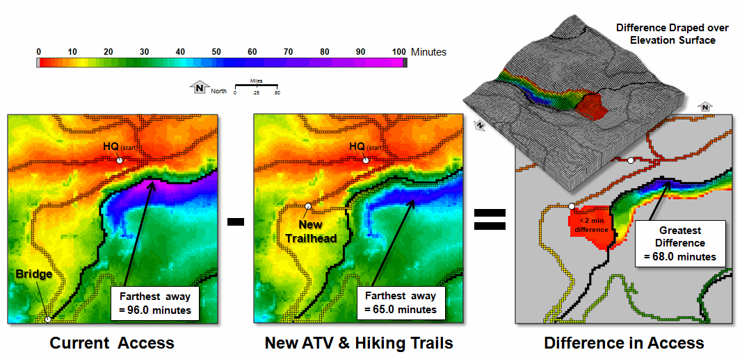
Figure 1. Subtracting two
travel-time surfaces determines the relative advantage at every location in a project
area.
The right side of figure
1 shows the difference in travel-time under current conditions and the proposed
new trail. This is accomplished by
simply subtracting the two maps—where 0 = unchanged response times (light grey),
values = difference in the response times (red through blue tones). The red area between the road and the
suspension bridge notes that ATV access is slightly improved (less than 2
minutes difference) with the introduction of the new trail. The greens and blues show considerable
improvement in response time with a maximum difference of 68.0 minutes.
Draping the result over
the elevation surface shows that the south side of the canyon bottom is best
serviced via the new trail. The more
important, non-intuitive information is the dividing line of best access
approach (red line) halfway up the southern side of the canyon. Locations nearer the top of the canyon are
best accessed via the current truck/ATV/Hiking utilizing the southern bridge.
Figure 2 extends the
analysis to characterize the optimal path for the most remote location under
current conditions. The first segment
(red) routes the truck along the road for approximately 19 minutes to an old
logging landing. The ATV’s are unloaded
and precede off-road (cyan) toward the northeast for an additional 15 minutes
(19 + 15= 34 minutes total). Note the
route’s “bend” to the east to avoid the sharply increased travel-time in the
rugged terrain along the west canyon rim as depicted in the travel-time
surface.
Once the southern side of
the canyon becomes too steep for the ATVs, the rescue team hikes the final
segment of 62 minutes (violet) for an estimated total elapsed time of 96
minutes (19 + 15 + 62 = 96). A digitized
routing file can be uploaded to a handheld GPS unit to assist off-road
navigation and real-time coordinates can be sent back to headquarters for
monitoring the team’s progress—much like commonplace network
navigation/tracking systems in cars and trucks, except on- and off-road
movement is considered.
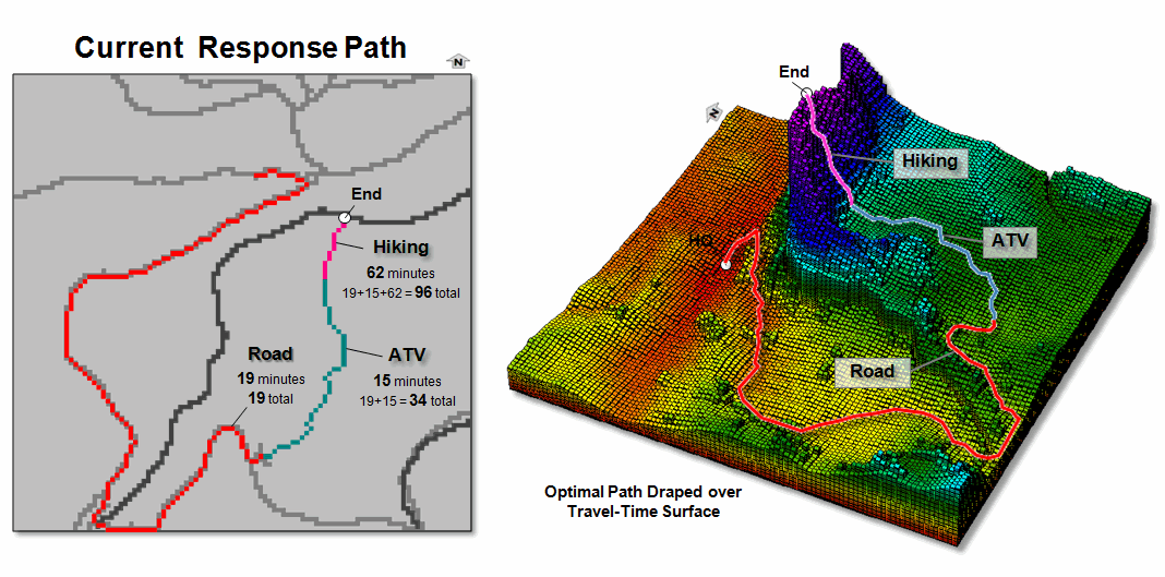
Figure 2. The optimal path is
identified as the steepest downhill route over a travel-time surface.
(see Author’s Note)
The backbone of the
backcountry emergency response model is the derivation of the travel-time
surface (right side of figure 2). It is
“calculated once and used many” as any location can be entered and the steepest
downhill path over the surface identifies the best response route from
headquarters—including Truck, ATV and Hiking segments with their estimated
lapsed times and progressive coordinates.
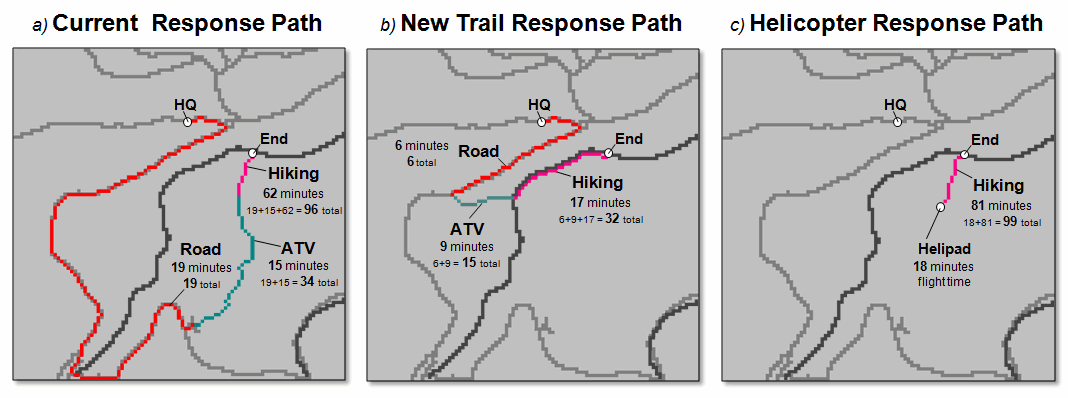
Figure 3. Comparison of emergency
response routes to a remote location under alternative scenarios.
In addition, alternate
scenarios can be modeled for different conditions, such as seasons, or proposed
projects. For example, figure 3 shows
three response routes to the same remote location—considering a) current
conditions, b) new trail and c) new helipad.
In this case, the response is much quicker for the new trail route
versus either the current or helipad alternatives.
It is important to note
that the validity of any spatial model is dependent on the quality of the
underlying data layers and the robustness of the model—garbage in (as well as
garbled throughput) is garbage out. In
this case, the model only considers one absolute barrier to movement (water)
and one relative barrier (slope) making it far too simplistic for operational
use. While it is useful for introducing
the concept, but considerable interaction between domain experts and GIS
specialists is needed to advance the idea into a full-fledged application …any
takers out there?
_____________________________
Author’s Note: See www.innovativegis.com/basis/MapAnalysis/Topic14/Topic14.htm#Hiking_time
for a more detailed discussion on deriving off-road travel-time surfaces and
establishing optimal paths.
Bringing
Travel and Terrain Directions into Line
(GeoWorld, December 2012)
The three previous
sections addressed “Backcountry 911” that considers both on- and off-road
travel for emergency response. As
identified in the left portion of figure 1, the analysis involves the
development of a “stepped accumulation surface” that first considers on-road
travel by assigning the minimum travel-time from headquarters to all of the
road locations. As shown in the figure,
the farthest away location considering truck travel is 26.5 minutes occurring
in the southeast corner of the project area.
The next step considers
disembarking anywhere along the road network and moving off-road by ATV. However, the ability to simulate different
modes of travel is not available in most grid-based map analysis toolsets. The algorithm requires the off-road movement
to “remember” the travel-time at each road location and then start accumulating
additional travel-time as the new movement twists, turns, and stops with
respect to the relative and absolute barriers calibrated for ATV off-road
travel (see Author’s Note 2).
The middle-left inset in
figure 1 shows the accumulated travel-time for both on-road truck and off-road
ATV travel where the intervening terrain conditions act like “speed limits”
(relative barriers). Also, ATV travel
is completely restricted by open water and very steep slopes (absolute
barriers). The result of the processing
assigns the minimum total travel-time to all accessible locations comprising
about 85% of the project area. The
farthest away location assuming combined truck and ATV travel is 52.1 minutes
occurring in the central portion of the project area.
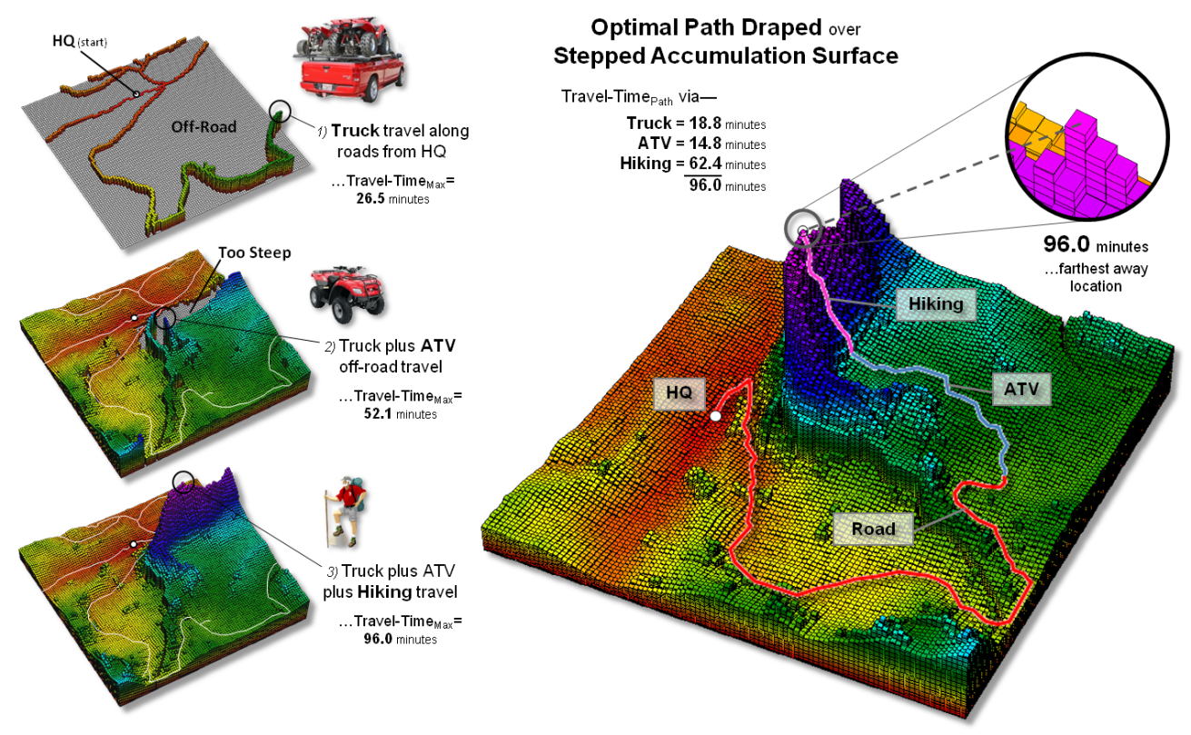
Figure 1. A backcountry emergency response surface identifies the travel-time of
the “best path” to all locations considering a combination of truck, ATV and
hiking travel.
The remaining 15% is too
steep for ATV travel and necessitates hiking into these locations. In a similar manner, the algorithm picks up
the accumulated truck/ATV travel-time values and moves into the steep areas
respecting the hiking difficulty under the adverse terrain conditions. Note the large increases in travel-time in
these hard to reach areas. The farthest
away location assuming combined truck, ATV and hiking is 96.0 minutes, also
occurring in the central portion of the project area.
A traditional
accumulation surface (one single step) identifies the minimum travel-time from
a starting location to all other locations considering “constant” definitions
of the relative and absolute barriers affecting movement. It has two very unique characteristics— 1) it
forms a bowl-like shape with the starting point (or points) having the lowest
value of zero = 0 units away from the start, and 2) continuously increasing
travel-time values reflecting the relative ease of movement that warps the bowl
with areas of relatively rapid increases in travel-time associated with areas
of high relative barrier “costs.”
A stepped accumulation
surface (top-center portion of figure 2) shares these characteristics but is
far more complex as it reflects the cumulative effects of different modes of
travel and the impact of their changing relative and absolute barriers on
movement. Note the dramatic “ridge”
running NE-SW through the center of the project area, as well as the other
morphological ups and downs in total combined travel-time.
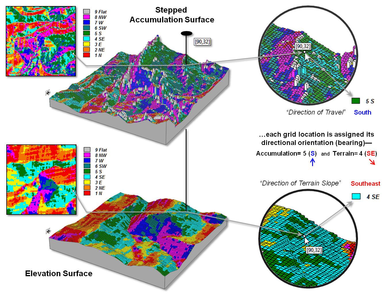
Figure 2. Maps of travel and terrain direction are characterized by the aspect
(bearings) of their respective surfaces.
In a sense, this
wrinkling is analogous to a terrain surface, but the surface’s configuration is
the result of the relative ease of on- and off-road travel in cognitive space—
not erosion, fracture, slippage and subsidence of dirt in real world
space.
However like a terrain surface,
an “aspect map” of the accumulation surface captures its orientation
information identifying the direction of the “best path” movement through every
grid location. The enlarged portion in
the top-right of the figure shows that the travel direction through location
90, 32 in the analysis frame is from the south (octant 5). The lower portion of the figure identifies
the terrain direction at the same location is oriented toward the southeast
(octant 4). Hence we know that the
movement through the location is across slope at an oblique uphill angle.
Figure 3 depicts a simple technique for combining the travel and
terrain direction information. A 2-digit
code is generated by multiplying “Travel Direction” map by 10 and adding it to
the “Terrain Direction” map. For
example, a “11” (one-one, not eleven) indicates that
movement is toward the north on a north-facing slope, indicating an aligned
downhill movement. A “15” indicates a
northerly movement up a south-facing slope.
The center inset in the figure
isolates all locations that have “aligned uphill movement” (opposing alignment)
in any of the cardinal directions indicated by 2-digit codes of 15, 26, 37, 48,
51, 62, 73, and 84. Locations having
“aligned downhill movement” are identified by codes of 11, 22, 33, 44, 55, 66,
77, and 88. All other combinations
indicate either oblique or orthogonal cross-slope movements, or locations
occurring on flat terrain without a dominant aspect.
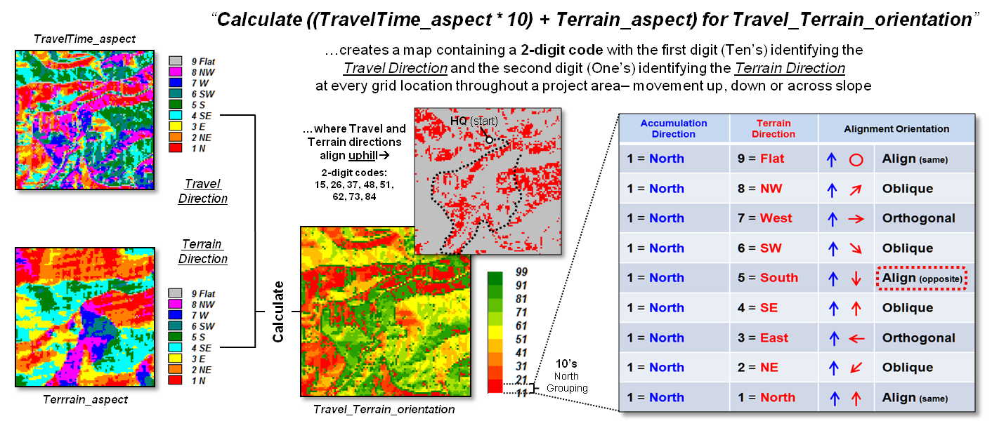
Figure 3. A 2-digit code is used to identify all combinations of travel and
terrain directions.
I realize the thought of
“an aspect map of an abstract surface,” such as a stepped accumulation surface
might seem a bit uncomfortable and well beyond traditional mapping; however it
can provide very “real” and tremendously useful information. Characterizing directional movement is not
only needed in backcountry emergency response but crucial in effective timber
harvest planning, wildfire propagation modeling, pipeline routing and a myriad
of other practical applications— such out-of-the-box spatial reasoning
approaches are what are driving geotechnology to a whole new plane.
_____________________________
Author’s
Note:
for a detailed discussion of “stepped accumulation surfaces,” see Topic 25,
calculating Effective Distance and Connectivity in the online book Beyond
Mapping III
posted at www.innovativegis.com/basis/MapAnalysis/.
Assessing
Wildfire Response (Part 1): Oneth by Land, Twoeth by Air
(GeoWorld, August 2011)
Wildfire initial attack
generally takes three forms: helicopter landing, helicopter
rappelling or ground attack.
Terrain and land cover conditions are used to determine accessible areas
and the relative initial attack travel-times for the three response modes. This and next month’s column describes GIS
modeling considerations and procedures for assessing and comparing alternative
response travel-times.
The discussion is based
on a recent U.S. Forest Service project undertaken by Fire Program Solutions
(see Author’s Notes). I was privileged
to serve as a consultant for the project that modeled the relative response
times for all of the Forest Service lands from the Rocky Mountains to the
Pacific Ocean—at a 30m grid resolution, that’s a lot of little squares. Fortunately for me, all I needed to do was
work on the prototype model, leaving the heavy-lifting and “practical
adjustments” to the extremely competent GIS specialist, wildfire professionals
and USFS helitack experts on the team. The objectives of the project were to model
the response times for different initial attack modes and provide summary maps,
tables and recommendations for strategic planning and management of wildfire
response assets.
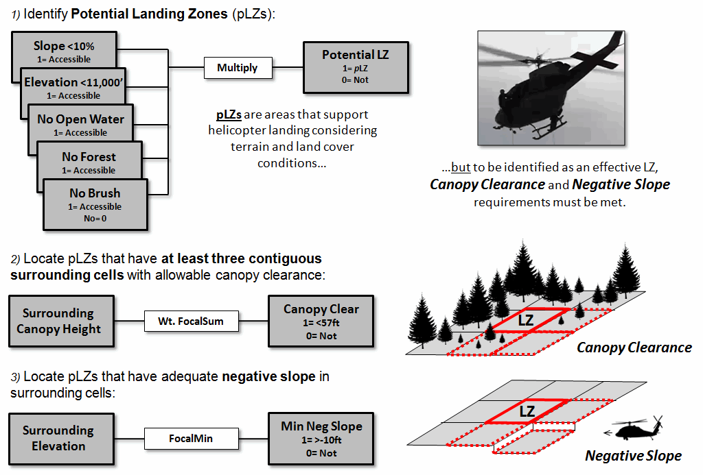
Figure 1. Generalized
outline of a grid-based model for identifying Potential Landing Zones (pLZs) that are further evaluated for helicopter
approach/departure considerations of Canopy Clearance and Negative Slope.
The most challenging
sub-model involved identifying helicopter landing zones (see figure 1). A simple binary suitability model is used to
identify Potential Landing Zones (pLZs) by assigning
a map value of 1 to all accessible terrain (gentle slopes and sub-alpine
elevations) and land cover conditions (no open water, forest or tall brush);
with 0 assigned to inaccessible areas.
Multiplying the binary set of maps derives a binary map of pLZs with 1 identifying locations meeting all of the
conditions (1*1*1*1*1= 1); 0 indicates locations with at least one
constraint.
Interior
locations of large contiguous pLZs groupings make
ideal landing zones. However, edge
locations or small isolated pLZs clusters must be
further evaluated for clear helicopter approach/departure flight paths. At least three contiguous cells surrounding a
pLZ must have forest canopy of less than 57 feet to
insure adequate Canopy Clearance. In addition, it is desirable to have a Negative Slope differential of at least
10 feet to aid landing and takeoff.
Two
steps are required for evaluating canopy clearance (see figure 2). A reclassify operation is used to calculate a
binary map with canopy heights of 57 feet or less assigned a value of 1; 0 for
taller canopies. A neighborhood
operation (FocalSum
in ArcGIS) is used to calculate the number of clear canopy cells in the
immediate vicinity of each pLZ cell (3x3 roving
window). If all cells are clear, a value
of 9 will be assigned, indicating an interior location in a grouping of pLZ cells.
For
derived values less than 9, an edge location or isolated pLZ
is indicated. If there are more than
four surrounding cells with adequate clearance, there has to be at least three
that are contiguous and the pLZ is assigned a map
value of 1 to indicate that there is a clear approach/departure; 0 for
locations with a sum of less than 4.
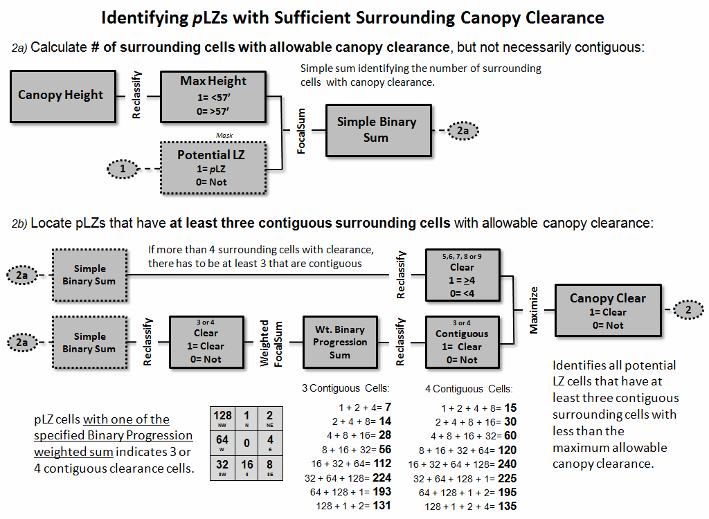
Figure 2. Procedure
for identifying pLZs with sufficient surrounding
canopy clearance.
Derived
values indicating 3 or 4 clear surrounding cells must be further evaluated to
determine if the cells are contiguous.
First, locations with a simple binary sum of 3 or 4 are assigned 1;
else= 0. A binary progression weighted
window—1,2,4,8,16,32,64,128—is used to generate a
weighted focal sum of the neighboring cells.
The weighted sum results in a unique value for all possible
configurations of the clear surrounding cells (see the lower portion of figure
2). For example, the only configuration
that results in a sum of 7 is the binary progression weights of 1+2+4
indicating contiguous cells N,NE,E.
The
weighted binary progression sums indicating contiguous cells are then
reclassified to 1; 0=else. Finally, the
minimum value for the “greater than 4 Clear” and “3 or 4 Clear” maps is taken
resulting in 1 for locations having sufficient contiguous canopy clearance
cells; else=0.
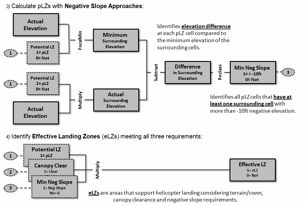
Figure 3. Procedures
for identifying pLZs with sufficient negative slope
(top) and combining all three considerations (bottom).
The top portion of figure
3 outlines the procedure for evaluating sufficient negative slope by
determining the difference between the minimum surrounding elevation and each pLZ elevation. If
the difference is greater than 10 feet, a map value of 1 is assigned; else= 0.
The final step multiplies
the binary maps of Potential LZ, Canopy Clearance and Minimum Negative
Slope. The result is a map of the
Effective LZs as 1*1*1= 1 for locations meeting all three criteria.
In the operational model,
the negative slope requirement was dropped as the client felt it was of
marginal importance. Next month’s column
will describe the analysis approaches for identifying ground response areas,
helicopter rappelling zones and the translation of all three response modes
into travel-time estimates for comparison.
_____________________________
Author’s Notes: For
more information on Fire Program Solutions and their wildfire projects contact
Don Carlton, DCARLTON1@aol.com.
Assessing
Wildfire Response (Part 2): Jumping Right into It
(GeoWorld, September 2011)
The previous section
noted that wildland fire initial attack generally takes three forms: helicopter
landing, helicopter rappelling or ground attack as determined
by terrain and land cover conditions (also “smoke-jumping” but that’s a
whole other story). The earlier
discussion described a spatial model developed by Fire Program Solutions (see
Author’s Notes) for identifying helicopter landing zones. The following discussion extends the analysis
to modeling and comparing the response times for the three different initial
attack modes for all locations within a project area.
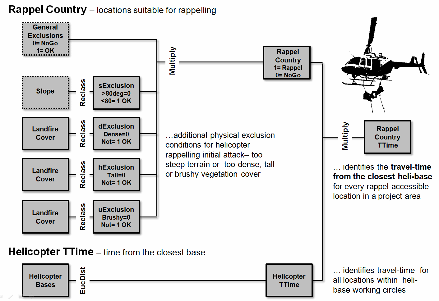
Figure 1. Major
steps and considerations in modeling wildfire Helicopter Rappel Attack
travel-time.
Figure 1 identifies the
major steps in determining “Rappel Country” …there are some among us so heroic
(crazy?) that they rappel out of a helicopter just to get to a wildfire before
the crowd. Rappel country is defined as
the areas where rappelling is the most effective initial attack mode based on
project assumptions. In addition to
general exclusions (e.g., open water, 10,000 foot altitude ceiling), rappelling
must consider four other highly variable physical exclusions— extremely steep
terrain (>80 degrees), very dense and/or tall forest canopies and dense tall
brush. The simple binary model in the
upper portion of figure 1 is used to identify locations suitable for rappelling
(1= OK; 0= NoGo) where the fearless can jump from a
hovering helicopter and slide down a rope between the trees up to a couple of
hundred feet to the ground.
The
lower portion of the figure uses a simple distance calculation to identify the
travel-time within a 75 mile working circle about a helibase assuming a defined
airspeed, round trip fuel capacity and other defining factors. By combining the binary map of rappel country
and the helicopter travel-time surface, an estimated travel-time from the
closest helibase to every Helicopter Rappelling Accessible location in a
project area is determined.
In
a similar “binary multiplication” manner, the helicopter travel-time to each
Effective Landing Zone can be calculated.
However, the landing crew must hike to a wildland fire outside the
landing zone. This secondary travel is
modeled in a manner similar to that used for the off-road movement of the
ground response model described below.
The helicopter flight time to a landing zone and the ground hiking time
to the fire are combined for an overall travel-time from the closest helibase
to every Helicopter Landing Accessible location in a project area.
Figure
2 outlines the major steps in modeling the combined on- and off-road response
time for a ground attack crew. On-road
travel is determined by the typical speed for different road types. The calculations for deriving the travel-time
to cross a 30m grid cell are shown in the rows of the table for five classes of
roads from major highways (R1) to backwoods roads (R5). Note that the slowest travel taking .1398
minute to traverse a backwoods road cell is over eight times slower than the
fastest (only .0172 min/cell).
Off-road
travel is based on typical hiking rates under increasingly steep terrain with
the steepest class (2.2369 min/cell) being 130 times slower than travel on a
highway. In addition, some locations
form absolute barriers to ground movement (e.g., very steep slopes, open
water).
The
three types of impedance are combined such that the minimum friction/cost value
is assigned to each location. A null
value is assigned to locations with absolute barriers. This composited friction (termed a Discrete Cost Surface) is used to
calculate the effective distance for every location to the closest dispatch
station. The procedure moves out from
each station in time step waves (like a stone tossed into a pond) that
considers the relative impedance as it propagates to generate an Accumulated
Cost Surface (TTime in minutes)
identifying the minimum travel-time from the closest initial dispatch location
to every location in a project area (see Author’s Notes).
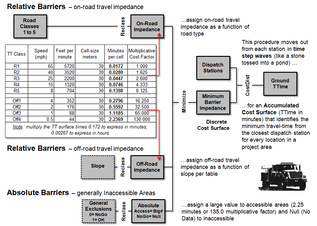
Figure 2. Major
steps and considerations in modeling wildfire Ground Attack travel-time.
The
three separate travel-time surfaces can be compared to identify the attack mode
with the minimum response time (see figure 3) and the differential times for
alternative attack modes. In operational
situations, this information could be accessed for a fire’s location and used
in dispatch and tactical planning.
In the “Rappel Country”
project the information is used for strategic planning of the arrangement of
helibase locations with rappel initial attack capabilities. Tabular summaries for travel-time from
existing helibases by terrain and land cover conditions were generated. In addition, rearrangement of helibase
location and capabilities could be simulated and evaluated.
From a GIS perspective
the project represents a noteworthy endeavor involving advanced grid-based map
analysis procedures over a large geographic expanse from the Rocky Mountains to
the Pacific Ocean that was completed in less than four months by a small team
of domain experts and GIS specialists.
The prototype analysis originally developed was interactively refined, modified
and enhanced by the team and then applied over the expansive area.
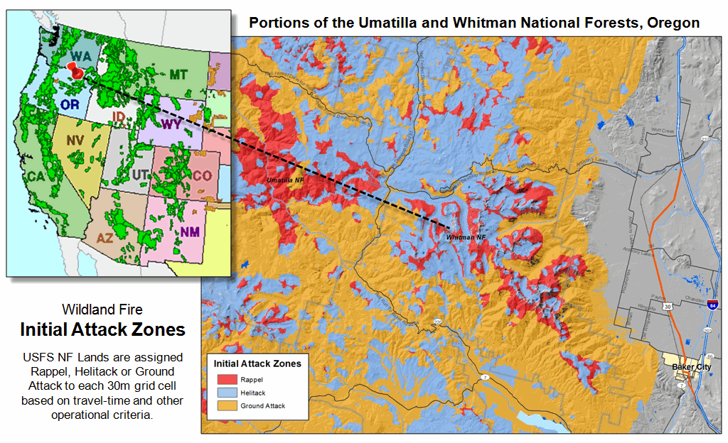
Figure 3. An example of a map of
the “best” initial attack mode for a fairly large area draped over a Google 3D
image.
As with most projects,
database development and model specification/parameterization formed the
largest hurdles—the grid-based map analysis component proved to be a
“piece-of-cake” compared to nailing down the requirements and slogging around
in millions upon millions of geo-registered 30m cells …whew!
_____________________________
Author’s Notes: For
more information on Fire Program Solutions, LLC and their wildfire projects
contact Don Carlton, DCARLTON1@aol.com;
for an in-depth discussion of travel-time calculation, see the online book Beyond
Modeling III, Topic 25, Calculating Effective Distance, posted at www.innovativegis.com/Basis/MapAnalysis/Default.htm.
Mixing It
up in GIS Modeling’s Kitchen
(GeoWorld, May 2013)
The modern “geotechnology recipe” is one part data,
one part analysis and a dash of colorful rendering. That’s a far cry from the historical mapping
recipe of basically all data with a generous ladling of cartography. Today’s maps are less renderings of “precise
placement of physical features for navigation and record-keeping” (meat and
potatoes) than they are interactive “interpretations of spatial relationships
for understanding and decision-making” (haute cuisine).
Figure 1 carries this cheesy cooking analogy a few
steps further. The left portion relates
our modern food chain to levels of mapped data organization from mouthfuls of
map values to data warehouses. The
center and right side of the figure ties these data (ingredients) to the GIS
modeling process (preparation and cooking) and display (garnishing and
presentation).
A map stack of geo-registered map layers is
analogous to a pantry that contains the necessary ingredients (map layers) for
preparing a meal (application). The meal
can range from Pop-Tart à la mode to the classic French coq au vin or Spain’s
paella with their increasing complexity and varied ingredients, but a recipe
all the same.
GIS Modeling is sort of like that but serves as
food for quantitative thought about the spatial relationships and patterns
around us. To extend the cooking
analogy, the rephrasing of an old saying seems appropriate— “Bits and bytes may
break my bones, but inaccurate modeling will surely poison me.” This suggests that while bad data can
certainly be a problem, ham-fisted processing of perfect data can spoil an
application just as easily.
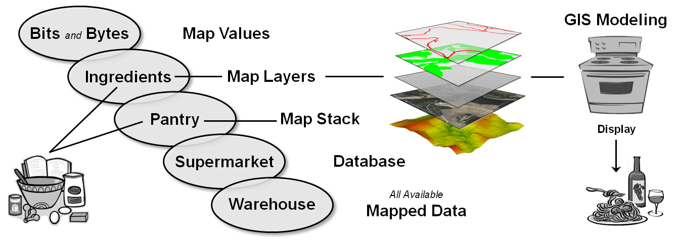
Figure 1. The levels of mapped data organization are
analogous to our modern food chain.
For example, a protective “simple distance buffer”
of a fixed distance is routinely applied around spawning streams that ignores
the relative erodibility of intervening terrain/soil/vegetation conditions
which can rain-down dirt balls that choke the fish in highly erodible palaces
and starve-out timber harvesting in places of low erodibility. In this case, the simple buffer is a
meager “rice-cake-like” solution that propagates at megahertz speed across the
mapping landscape helping neither the fish nor the logger. A more elaborate recipe involving a “variable-width
buffer” is needed, but it is rarely employed.
GIS tends to focus a great deal on spatial data
structure, formats, characteristics, query and visualization, but less on the
analytical processing that “cooks” the data (meant in the most positive
way). So what are the fundamental
considerations in GIS models and modeling?
How does it relate to traditional modeling?
At the highest conceptual level, GIS modeling has
two important characteristics—processing structure and elemental
approaches. The center portion of figure
2 depicts the underlying Processing Structure for all
quantitative data analysis as a progression from fundamental operations
to generalized techniques to key sub-models and finally to full
application models.
This traditional mathematical structure uses
sequential processing of basic math/stat operations to perform a wide variety
of complex analyses. By controlling the
order in which the operations are executed on variables, and using common
storage of intermediate results, a robust and universal mathematical processing
structure is developed.
The "map-ematical"
structure is similar to traditional algebra in which primitive operations, such
as addition, subtraction, and exponentiation, are logically sequenced for
specified variables to form equations and models. However in map algebra 1) the variables
represent entire maps consisting of geo-registered sets of map values, and 2)
the set of traditional math/stat operations are extended to simultaneously
evaluate the spatial and numeric distributions of mapped data.
Each processing step is accomplished by requiring—
- retrieval of one or more map
layers from the map stack,
- manipulation of that mapped data
by an appropriate math/stat operation,
- creation of an intermediate
map layer whose map values are derived as a result of that manipulation,
and
- storage of that new map layer back into the map stack for subsequent
processing.
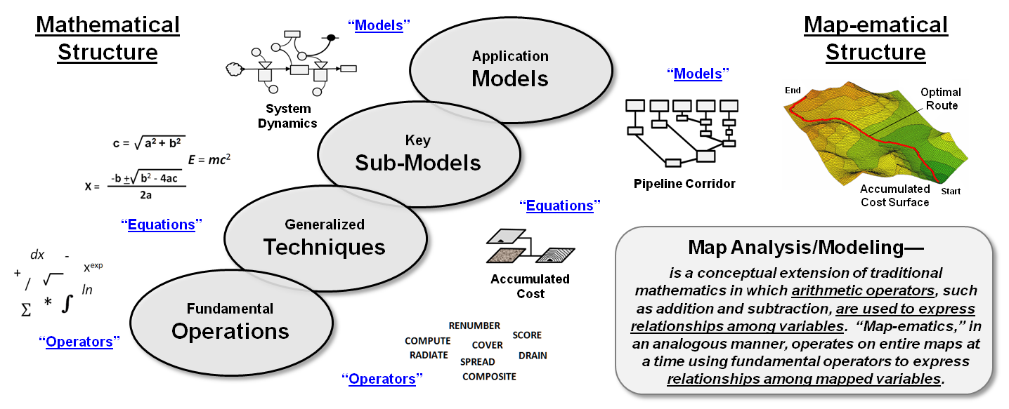
Figure 2. The
"map-ematical structure" processes entire
map layers at a time using fundamental operators to express relationships among
mapped variables in a manner analogous to our traditional mathematical
structure.
The
cyclical nature of the retrieval-manipulation-creation-storage processing
structure is analogous to the evaluation of “nested parentheticals” in
traditional algebra. The logical
sequencing of map analysis operations on a set of map layers forms a spatial model
of specified application. As with
traditional algebra, fundamental techniques involving several primitive
operations can be identified that are applicable to numerous situations.
The
use of these primitive map analysis operations in a generalized modeling
context accommodates a variety of analyses in a common, flexible and intuitive
manner. Also it provides a framework for
understanding the principles of map analysis that stimulates the development of
new techniques, procedures and applications (see author’s note 1).
The
Elemental
Approaches
utilized in map analysis and GIS modeling also are rooted in traditional
mathematics and take on two dimensions— Atomistic/Analysis versus
Holistic/Synthesis.
The Atomistic/Analysis approach to GIS
modeling can be thought of as “separating a whole into constituent elements”
to investigate and discover spatial relationships within a system (figure
3). This “Reductionist’s approach” is
favored by western science which breaks down complex problems into simpler
pieces which can then be analyzed individually.
The Holistic/Synthesis approach, in
contrast, can be thought of as “combining constituent elements into a whole”
in a manner that emphasizes the organic or functional relationships between
the parts and the whole. This “Interactionist’s approach” is often associated with eastern
philosophy of seeing the world as an integrated whole rather than a dissociated
collection of parts.
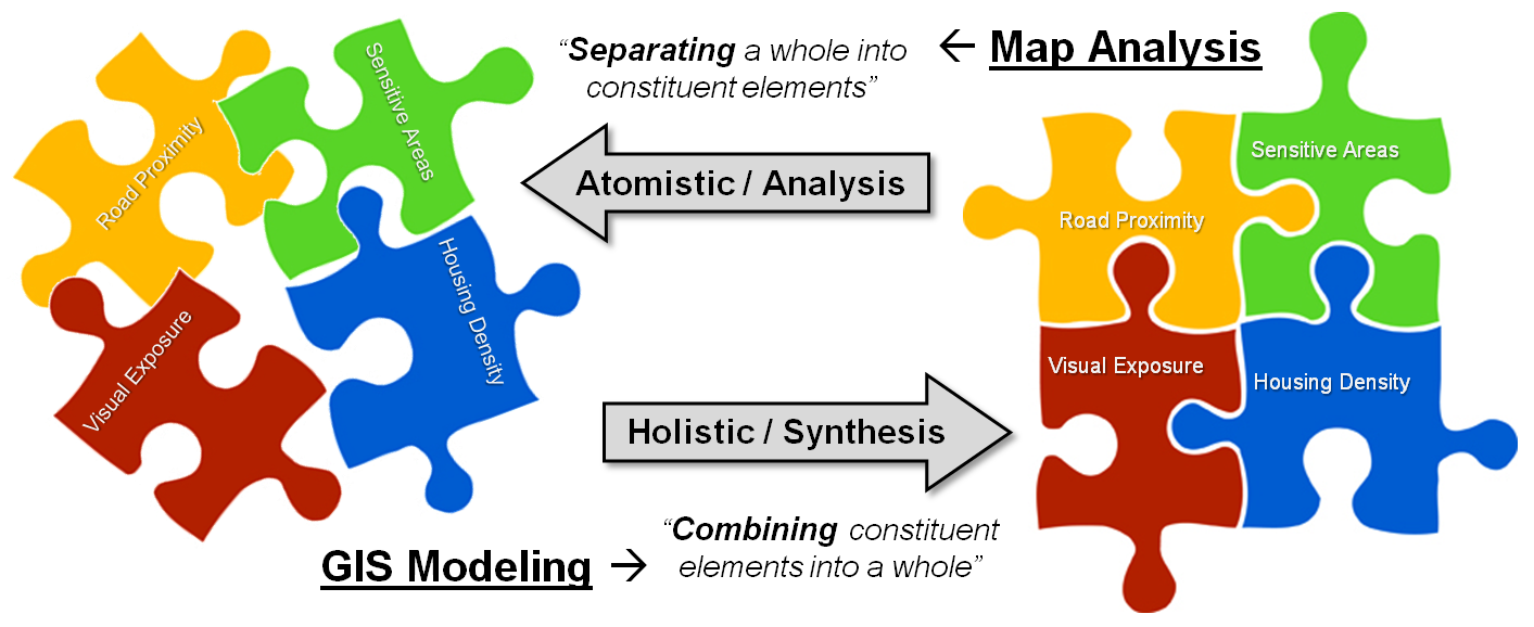
Figure 3. The two Elemental Approaches utilized in map
analysis and GIS Modeling.
So what does all this have to do with map analysis
and GIS modeling? It is uniquely
positioned to change how quantitative analysis is applied to complex real-world
problems. First, it can be used account
for the spatial distribution as well as the numerical distribution inherent in
most data sets. Secondly, it can be used
in the atomistic analysis of spatial systems to uncover relationships among
perceived driving to variables of a system.
Thirdly, it can be used in holistic synthesis to model changes in
systems as the driving variables are altered or generate entirely new
solutions.
In a sense, map analysis and modeling are like chemistry. A great deal of science is used to break down
compounds into their elements and study the interactions—atomistic/analysis.
Conversely, a great deal of innovation is used to assemble the elements into new
compounds— holistic/synthesis. The combined
results are repackaged into entirely new things from food additives to cancer
cures.
Map analysis and GIS modeling operate in an analogous manner. They use many of the same map-ematical operations to first analyze and then to synthesize
map variables into spatial solutions from navigating to a new restaurant to
locating a pipeline corridor that considers a variety of stakeholder
perspectives. While dictionaries define
analysis and synthesis as opposites, it is important to note that in geotechnology,
analysis without synthesis is almost worthless …and that the converse is just
as true.
_____________________________
Author’s Notes: 1) see the discussion of the SpatialSTEM approach
in Topic 30, “A Math/Stat Framework for
Map Analysis” posted at www.innovativegis.com/basis/MapAnalysis/Topic30/Topic30.htm. 2) For more on GIS models and modeling, see
the GeoWorld series of Beyond Mapping columns (January,
February and December 1995) in the online book Beyond Mapping II, Topic 5, “A
Framework for GIS Modeling” posted at www.innovativegis.com/basis/BeyondMapping_II/Topic5/BM_II_T5.htm.
Putting GIS Modeling Concepts in Their Place
(GeoWorld, October 2010)
The vast majority of GIS
applications focus on spatial inventories that keep track of things, characteristics
and conditions on the landscape— mapping and geo-query of Where is What. Map analysis and GIS modeling applications,
on the other hand, focus on spatial relationships within and among map layers— Why,
So What and What If.
Natural resource fields
have a rich heritage in GIS modeling that tackles a wide range of management
needs from habitat mapping to land use suitability to wildfire risk assessment
to infrastructure routing to economic valuation to policy formulation. But before jumping into a discussion of GIS
analysis and modeling in natural resources it seems prudent to establish basic
concepts and terminology usually reserved for an introductory lecture in a
basic GIS modeling course.
Several years ago I
devoted a couple of Beyond Mapping columns to discussing the various types and
characteristics of GIS models (see Author’s note). Figure 1 outlines this typology with a bit of
reorganization and a few new twists and extensions gained in the ensuing 15
years. The dotted connections in the
figure indicate that the terms are not binary but form transitional gradients,
with most GIS models involving a mixture of the concepts.
Simply stated any model
is a representation of reality in either material form (tangible
representations) or symbolic form (abstract representations). The two general types of models include
structural and relational. Structural
models focus on the composition and construction of tangible things and
come in two basic forms— action involving dynamic movement-based models,
such as a model train along its track and object involving static
entity-based models forming a visual representation of an item, such as an
architect’s blueprint of a building. CAD
and traditional GIS inventory-oriented applications fall under the “object”
model type.
Relational models, on the other hand, focus on the interdependence
and relationships among factors. They
come in two types— functional models based on input/output that track
relationships among variables, such as storm runoff prediction and conceptual
models based on perceptions that incorporate fact interpretation and value
weights, such as suitable wildlife habitat derived by interpreting a stack of
maps describing a landscape.
Fundamentally there are
two types of GIS models—cartographic and spatial. Cartographic models automate manual
techniques that use traditional drafting aids and transparent overlays (i.e., McHarg overlay), such as identifying locations of
productive soils and gentle slopes using binary logic expressed as a
geo-query. Spatial models express
mathematical and statistical relationships among mapped variables, such as
deriving a surface heat map based on ambient temperature and solar irradiance
involving traditional multivariate concepts of variables, parameters and
relationships.
All GIS models fall under
the general “symbolic --> relational” model types, and because digital maps
are “numbers first, pictures later,” map analysis and GIS modeling are usually
classified as mathematical (or maybe that should be “map-ematical”). The somewhat subtle distinction between
cartographic and spatial models reflects the robustness of the map values and
the richness of the mathematical operations applied.
The general
characteristics that GIS models share with non-spatial models include purpose,
approach, technique and temporal considerations. Purpose identifies a model’s
intent/utility and often involves a descriptive characterization of the
direct interactions of a system to gain insight into its processes, such as a
wildlife population dynamics map generated by simulation of life/death
processes. Or the purpose could be prescriptive
to assess a system’s response to management actions/interpretations, such as
changes in a proposed power line route under different stakeholder’s
calibrations and weights of input map layers.
A model’s Approach
can be empirical or theoretical. An empirical
model is based on the reduction (analysis) of field-collected measurements,
such as a map of soil loss for each watershed for a region generated by
spatially evaluating the empirically derived Universal Soil Loss equation. A theoretical model, on the other
hand, is based on the linkage (synthesis) of proven or postulated relationships
among variables, such as a map of spotted owl habitat based on accepted
theories of owl preferences.
![]()
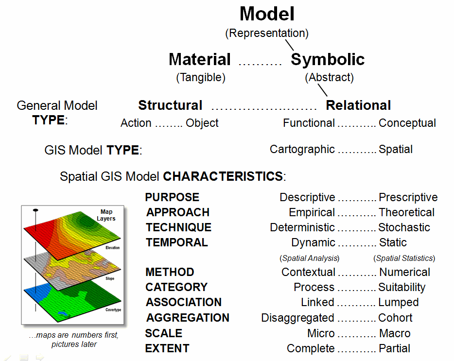
Figure 1. Types
and characteristics of GIS models.
Modeling Technique
can be deterministic or stochastic. A deterministic
model uses defined relationships that always results in a single repeatable
solution, such as a wildlife population map based on one model execution using
a single “best” estimate to characterize each variable. A stochastic model uses repeated
simulation of a probabilistic relationship resulting in a range of possible
solutions, such as a wildlife population map based on the average of a series
of model executions.
The Temporal
characteristic refers to how time is treated in a model— dynamic or
static. A dynamic model treats
time as variable and model variables change as a function of time, such as a
map of wildfire spread from an ignition point considering the effect of the
time of day on weather conditions and fuel loading dryness. A static model treats time as a
constant and model variables do not vary over time, such as a map of timber
values based on the current forest inventory and relative access to roads.
The modeling Method,
however, is what most distinguishes GIS models from non-spatial models by
referring to the spatial character of the processing— contextual or
numerical. Contextual methods use
spatial analysis to characterize “contextual relationships” within and among
mapped data layers, such as effective distance, optimal paths, visual
connectivity and micro-terrain analysis.
Numerical methods use spatial statistics to uncover “numerical
relationships” within and among mapped data layers, such as generating a
prediction map of wildfire ignition based regression analysis of historical
fire occurrence and vegetation, terrain and human activity map layers.
Spatial Analysis (contextual spatial relationships) and Spatial
Statistics (numerical spatial relationships) form the “toolboxes” that are
uniquely GIS and are fueling the evolution from descriptive mapping and “geo-query”
searches of existing databases to investigative and prescriptive map
analysis/modeling that address a variety of complex spatial problems— a
movement in user perspective from “recordkeeping” to “solutions.”
The Category
characteristic of GIS models is closely related to the concept of “Relational”
in general modeling but speaks specifically to the type of spatial
relationships and interdependences among map layers. A process-oriented model involves
movement, flows and cycles in the landscape, such as timber harvesting access
considering on- and off-road movement of hauling and harvesting equipment. A suitability-oriented model
characterizes geographic locations in terms of their relative appropriateness
for an intended use.
Model association,
aggregation, scale and extent refer to the geographic nature of how map layers
are defined and related. Association
refers to how locations relate to each other and can be classified as lumped
when the state/condition of each individual location is independent of other
map locations (i.e., point-by-point processing). A linked association, on the other
hand, occurs when the state/condition of each individual location is dependent
on other map locations (i.e., vicinity, neighborhood or regional processing).
Aggregation describes the grouping of map locations for
processing and is termed disaggregated when a model is executed for each
individual spatial object (usually a grid cell), such as in deriving a map of
predicted biomass based on spatially evaluating a regression equation in which
each input map layer identifies an independent “variable,” each location a
“case,” and each map value a “measurement” as defined in traditional statistics
and mathematical modeling.
Alternatively, cohort
aggregation utilizes groups of spatial objects having similar characteristics,
such as deriving a timber growth map for each management parcel based on a
look-up table of growth for each possible combination of map layers. The model is executed once for each combination
and the solution is applied to all map locations having the same “cohort”
combination.
GIS modeling
characteristics of Scale and Extent retain their traditional
meanings. A micro scale model
contains high resolution (level of detail) of space, time and/or variable
considerations governing system response, such as a 1:1,000 map of a farm with
crops specified for each field and revised each year. A macro scale model contains low
resolution inputs, such as a 1:1,000,000 map of land use with a single category
for agriculture revised every 10 years.
A GIS model’s Extent
is termed complete if it includes the entire set of space, time and/or
variable considerations governing system response, such as a map set of an
entire watershed or river basin. A partial
extent includes subsets of input data that do not completely cover an area of
interest, such as a standard topographic sheet with its artificial boundary
capturing limited portions of several adjoining watersheds.
For those readers who are
still awake, you have endured an introductory academic slap and now possess all
of the rights, privileges and responsibilities of an introductory GIS modeling
expert who is fully licensed to bore your peers and laypersons alike with such
arcane babble. Next month’s discussion
will apply and extend these concepts to model logic, degrees of abstraction,
levels of analysis and processing levels using an example model for assessing
campground suitability.
_____________________________
Author’s Note: If
you have old GW magazines lying about, see “What’s in a Model?” and “Dodge the
GIS Modeling Babble Ground” in the January and February 1995 issues of GIS
World (the earlier less inclusive magazine name for GeoWorld) or visit www.innovativegis.com, Beyond Mapping
III, Chronological Listing, and scroll down to the Beyond Mapping II online
compilation of Beyond Mapping columns from October 1993 to August 1996 that is
in back-burner preparation.
A Suitable Framework for GIS Modeling
(GeoWorld, November 2010)
Suitability Modeling is
one of the simplest and most frequently used GIS modeling approaches. These models consider the relative “goodness”
of each map location for a particular use based on a set of criteria. For example, figure 1 outlines five Criteria
considerations for locating a campground: favor gentle terrain, being near
roads and water, with good views of water and oriented toward the west.
In the flowchart of the
model’s logic, each consideration is identified as a separate “row.” In essence every map location is graded in
light of its characteristics or conditions in a manner that is analogous to a professor
evaluating a set of exams during a semester.
Each spatial consideration (viz. exam) is independently graded (viz.
student answers) with respect to a consistent scale (viz. an A to an F
grade).
Figure 2 identifies Analysis
Levels as “columns” used to evaluate each of the criteria and then combines
them into an overall assessment of campground suitability. Base Maps represent the physical
characteristics used in the evaluations— maps of Elevation, Roads, and Water in
this case. But these “facts” on the
landscape are not in a form that can be used to evaluate campground
suitability.
![]()
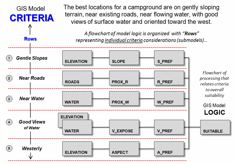
Figure 1. Campground Suitability model logic with rows indicating
criteria.
Derived Maps translate physical descriptions into suitability
contexts. For example, it is not
Elevation per se that affects campground suitability, but the rate and
direction of the change in elevation expressed as Slope and Aspect that
characterize terrain configuration.
Similarly, it is not the presence of roads and water but the relative
closeness to these features that affects the degree of suitability (Prox_R and Prox_W).
Interpreted Maps identify increasing abstraction from Facts on the
landscape to Judgments within the context of suitability. At this level, derived maps are
interpreted/graded into a relative suitability score, usually on a scale from 1
(least suitable/worst) to 9 (most suitable/best). Using the exam grading analogy, a map
location could be terrible in terms of terms of proximity to roads and water
(viz. a couple of F’s on two of the exams) while quite suitable in terms of
terrain steepness and aspect (viz. A’s on two other exams).
Like a student’s semester
grade, the overall suitability, or Combined Map, for a campground is a
combination of the individual criteria scores.
This is usually accomplished by calculating the simple or
weighted-average of the individual scores.
The result is a single value indicating the overall “relative goodness”
for each map location that in aggregate forms a continuous spatial distribution
of campground suitability for a given project area.
However, some of the
locations might be constrained by legal or practical concerns that preclude
building a campground, such as very close to water or on very steep
terrain. A Constraint Map
eliminates these locations by forcing their overall score to “0”
(unsuitable).
![]()
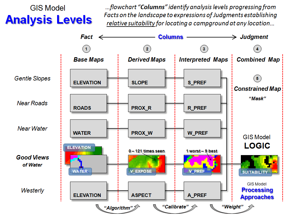
Figure 2. Flowchart
columns represent analysis levels transforming facts into judgment.
The logical progression
from physical Facts to suitability Judgments involves four basic Processing
Approaches— Algorithm, Calibrate, Weight, and Mask. For example, consider the goal of “good views
of water.” The derived map of visual
exposure to water (V_Expose) uses an Algorithm
that counts the number of times each location is visually connected to water
locations—
RADIATE Water OVER Elevation TO 100 AT 1 Completely FOR V_Expose
…that in this example,
results in values from 0 to 121 times seen.
In turn, the visual exposure map is Calibrated
to a relative suitability scale of 1 (worst) to 9 (best)—
RENUMBER V_Expose ASSIGNING 9 TO 80
THRU 121 ASSIGNING 8 TO 30 THRU 80 ASSIGNING 5 TO 10 THRU 30 ASSIGNING 3 TO 6 THRU 10 ASSIGNING 1 TO 0 THRU 6 FOR V_Pref
The interpreted visual exposure
map and the other interpreted maps are Weighted
by using a simple arithmetic average—
ANALYZE S_PREF TIMES 1 WITH W_PREF TIMES 1 WITH V_Pref
TIMES 1 WITH A_PREF TIMES 1 WITH R_PREF TIMES 1 Mean FOR Suitable
Finally, a binary constraint
map (too steep and/or too close to water = 0; else= 1) is used to Mask
unsuitable areas—
COMPUTE Suitable Times Constraints FOR Suitable_masked
Figure 3 depicts the Processing
Flow as a series of map analysis operations/commands. You are encouraged to follow the flow by
delving into more detail and even complete a hands-on exercise in suitability
modeling (see author’s note)— it ought to be a lot of
fun, right?
![]()
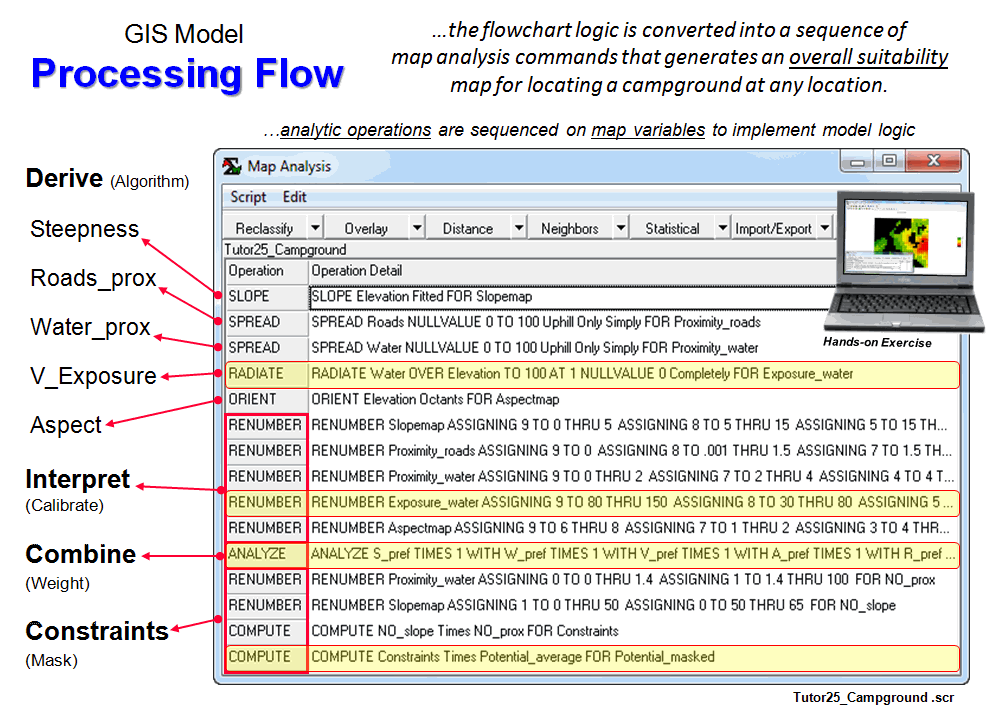
Figure 3. Processing flow that implements
the Campground Suitability model.
_____________________________
Author’s Note: An
annotated step-by-step description of the Campground Suitability model and
hands-on exercise materials are posed at www.innovativegis.com/basis/Senarios/Campground.htm. Additional discussion of types and approaches
to suitability modeling is posted at www.innovativegis.com/basis/MapAnalysis/Topic23/Topic23.htm.
GIS’s Supporting Role in the Future of Natural Resources
(GeoWorld, December 2010)
My completely charming
wife recently made a thought-provoking presentation entitled “Human Dimensions:
From Backstage to Front and Center” for a seminar series on Decades of Change
in Ecological Research at Colorado State University. In the talk she made reference that in 1970s
individual disciplinary scientists controlled the podium of discussion, and
social science, its issues and human dimensions, were primarily back stage in
natural resource research, planning and management (left side of figure
1).
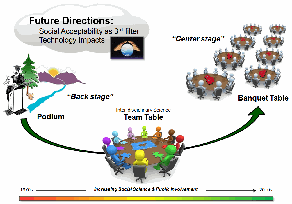
Figure 1. Social science and human
dimensions in natural resources have moved from back stage to front and center.
In the 1980s, the podium
became a “team table” with a diversity of disciplines collaboratively engaged in
science-based discussion for assessing management options. The discussion around the table was expanded
to include social science’s theories and understandings of human values,
attitudes and behaviors.
During the 1990s, the team
table expanded further to a room full of “banquet tables” containing a broad
diversity of interests promoting direct and active engagement of scientists,
managers, stakeholders and representative publics in the conversation. The interaction was space/time bound to
scheduled meetings, representative input, organized discussion and manual flip
chart documentation.
What dramatically changed
over the years is the role of human dimensions in addressing natural resource
issues from its early “back stage” position to a “front and center” involvement
and increasingly active voice. Today and
into the future, Social Acceptability has fully joined Ecosystem
Sustainability and Economic Viability as a critical third filter
needed for successful decision-making (figure 2). Like a three-legged stool, removal of any of
the legs results in an unstable condition and the likelihood of failed
decisions.
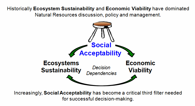
Figure 2. Social acceptability of
plans and policy has become an important third filter in natural resources
management.
Joining social
acceptability as a significant factor impacting the future of natural resources
is the changing capabilities and roles of technology— with geotechnology poised
to play a key supporting role.
Spatially-enabled Social Networking concepts, such as “community
collaborative mapping,” “participatory GIS,” “user generated content” and the
“spatial tweet” will be the shared futures of social science, natural resources
and geotechnology.
To a large extent, GIS
technology had a fairly slow start in natural resources as practical
application got mired in the forest mensuration and mapping units within most
NR organizations— data first, utility later.
While innovative research projects demonstrated new ways of doing
business with spatial data, the data-centric perspective of the specialists
(mapping and geo-query) dominated the analysis-centric needs of the managers,
policy and decision makers (spatial reasoning and modeling).
But with the growing
voice of human dimensions in natural resources there appears to be a plot twist
in the works. Maps are being viewed less
and less as static wall hangings depicting “where is what” and more as
dynamic spatial expressions of “why, so what and what if…” within the
context of alternative management and policy options.
That brings us to one of
the hottest new things in computing… “crowdsourcing.” In case some of you (most?) might not be
aware of this new field, a thumbnail sketch with a bit of discussion seems in
order (figure 3). Crowdsourcing
is a term that mashes the words "crowd" and "outsourcing"
to describe the act of taking tasks traditionally performed by a team of
in-house or outsourced specialists, and outsourcing the tasks to the community
through an ‘open call’ to a large group of people (the crowd) asking for their
input (Wikipedia).
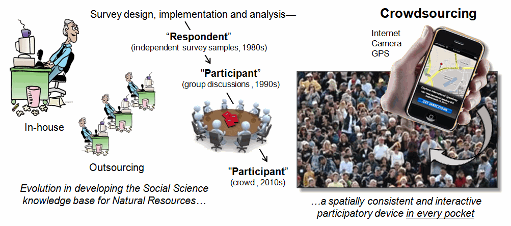
Figure 3. Crowdsourcing solicits
mass collaboration via the Internet in formulating socially acceptable policy
and plans.
For example, the public may
be invited to carry out a design task (also known as “community-based design”
and “distributed participatory design”), or help capture, systematize or
analyze large amounts of data (citizen science) by leveraging mass
collaboration enabled by the Internet.
Many cities now provide a
smart phone “app” for citizens to take a picture of a pothole and send the
geo-tagged photo to the streets department.
In a similar manner, park users could report hiking trail locations in
need of repair, rate their of trail experience or even send pictures of areas
they believe are unusually beautiful or ugly.
Crowdsourcing simply provides a modern mechanism for completing a survey
in digital form while in route or when they get back to the parking lot and
civilized connectivity.
However for natural
resource professionals and GIS’ers, crowdsourcing can go well beyond data
collection by extending the “social science tools” for consensus building and
conflict resolution used in calibrating and weighting spatial models. For example, a model for routing an electric
transmission line that considers engineering, environmental and development
factors can be executed under a variety of scenarios reflecting different
influences of the criteria map layers as interpreted by different stakeholder
groups (see Author’s Note). The result
is infusion of the collective interpretation and judgment required for
effective cognitive mapping—participatory input.
Currently, the
calibrating and weighting a spatial model usually involves a small set of
representatives sitting around a table and hashing out a presumed collective
opinion of a larger group’s understanding, interpretations and relative
weightings. Crowdsourcing suggests one
can hang a routing or other spatial model out on a website, invite folks to
participate, have some GUI’s that let them interactively set the model’s
calibrations and weights, and then execute their scenario. They could repeat as often as they like, and
once satisfied with a solution they would submit the model parameters. Sort of a virtual public hearing but with
more refined interaction and less stale doughnuts and lukewarm coffee left on
the tables.
To
complete the playhouse metaphor, mapping and geo-query will set the stage, while
spatial reasoning and modeling plays out the production with the active
participation of an extended audience of scientists, managers, stakeholders and
publics—sort of a natural resources experimental theater in the round. This ought to be fun with human dimensions
front and center in the limelight and geotechnology handling the stage
management.
_____________________________
Author’s Note: For a discussion of procedures in participatory GIS see the online
book, Beyond Mapping III, Topic
19, “A Recipe for Calibrating and Weighting