Beyond Mapping III
|
Map
Analysis book with companion CD-ROM
for hands-on exercises and further reading |
Suitability Models Find the Good,
the Bad and the Hugag — describes
a simple suitability model for characterizing habitat
Mapping Techniques Rate Hugag Habitat Suitability — expands
discussion to Binary Progression and Rating suitability models
Logic and Extent Elevate Suitability Models
to New Levels — extends
Rating discussion to include additional habitat considerations and model
weighting
Breaking Away from Breakpoints — describes
the use of curve-fitting to derive continuous equations for suitability model
ratings
Extended Experience Materials — provides hands-on experience with Suitability Modeling
Note: The processing and figures
discussed in this topic were derived using MapCalcTM
software. See www.innovativegis.com to download a free
MapCalc Learner version with tutorial materials for classroom and self-learning
map analysis concepts and procedures.
<Click here> right-click to download a
printer-friendly version of this topic (.pdf).
(Back to the Table of Contents)
______________________________
Suitability
Models Find the Good, the Bad and the Hugag
(GeoWorld, July 2004, pg. 20-21)
A simple
habitat model can be developed using only reclassify and overlay
operations. For example, a Hugag is a curious mythical beast (see figure 1) with
strong preferences for terrain configuration:
¾ Prefers
low elevations (severe nose bleeds
at higher altitudes)
¾ Prefers
gentle slopes (fear of falling over
and unable to get up)
¾ Prefers
southerly aspects (a place in the
sun)
A
binary habitat model of Hugag preferences is the
simplest to conceptualize and implement.
It is analogous to the manual procedures for map analysis popularized in
the book Design with Nature, by Ian
L. McHarg, first published in 1969. This seminal work was the forbearer of modern
map analysis by describing an overlay procedure involving paper maps,
transparent sheets and pens.
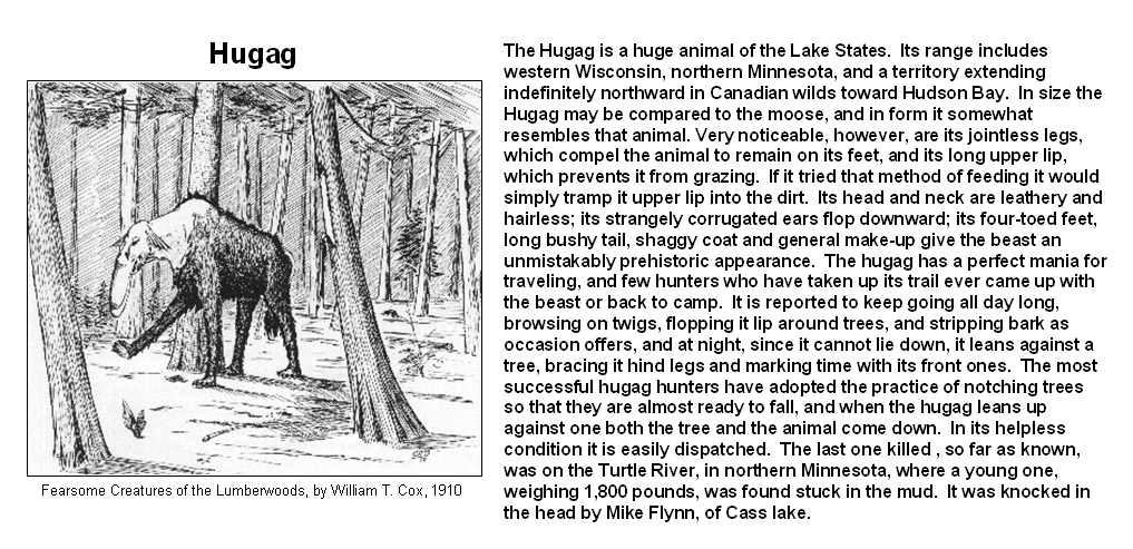
Figure
1. The Hugag prefers
low elevations, gentle slopes and southerly aspects.
(see http://www.fearsomecreaturesofthelumberwoods.com/mainindex.htm
for more fearsome creatures)
For
example, if avoiding steep slopes was an important decision criterion, a
draftsperson would tape a transparent sheet over a topographic map, delineate
areas of steep slopes (contour lines close together) and fill-in the
precipitous areas with an opaque color.
The process is repeated for other criteria, such as the Hugag’s preference to avoid areas that are
northerly-oriented and at high altitudes.
The annotated transparencies then are aligned on a light-table and the
“clear” areas showing through identify acceptable Hugag
habitat.
An
analogous procedure can be implemented in a computer by using the value 0 to
represent the
unacceptable areas (opaque) and 1 to represent acceptable habit
(clear). As shown in figure 2, an Elevation map is used to derive a map of
terrain steepness (Slope_map)
and orientation (Aspect_map). A value of 0 is assigned to locations Hugags want to avoid—
Greater
than 1800 feet elevation = 0 …too high
Greater
than 30% slope = 0 …too steep
North,
northeast and northwest = 0 …to northerly
—with
all other locations assigned a value of 1 to indicate acceptable areas.
The
individual binary habit maps are shown in 3D and 2D displays on the right side
of figure 2. The dark red portions
identify unacceptable areas that are analogous to McHarg’s
opaque colored areas delineated on otherwise clear transparencies.
A Binary
Suitability map of Hugag habitat is generated
by multiplying the three individual binary preference maps (left side of figure
3). If a zero is encountered on any of
the map layers, the solution is sent to zero (bad habitat). For the example location on the right side of
the figure, the preference string of values is 1 * 1 * 0 = 0 (Bad). Only locations with 1 * 1 * 1 = 1 (Good)
identify areas with out any limiting factors—good
elevations, good slopes and good orientation.
These areas are analogous to clear areas showing through the stack of
transparencies.
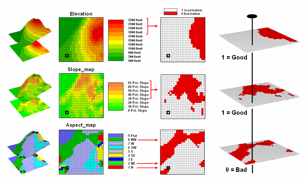
Figure
2. Binary maps representing Hugag
preferences are coded as 1= good and 0= bad.
While
this procedure mimics manual map processing, it is limited in the information
it generates. The solution is binary and
only differentiates acceptable and unacceptable locations. But isn’t an area that is totally bad (0 * 0
* 0 = 0) different from one that is just limited by one factor (1 * 1 * 0 =
0)? Two factors are acceptable thus
making it “nearly good.”
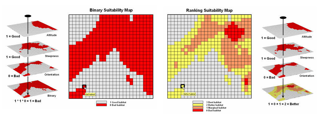
Figure
3. The binary habitat maps are multiplied
together to create a Binary Suitability map (good or bad) or added together to
create a Ranking Suitability map (bad, marginal, better or best).
The
right side of figure 3 shows a Ranking Suitability map of Hugag habitat. In
this instance the individual binary maps are simply added together for a count
of the number of acceptable locations.
Note that the areas of perfectly acceptable habitat (light grey) on both
the binary and ranking suitability maps have the same geographic pattern. However, the unacceptable area on the ranking
suitability map contains values 0 through 2 indicating how many acceptable
factors occur at each location. The zero
value for the area in the northeastern portion of the map identifies very bad
conditions (0 + 0 + 0= 0). The example
location, on the other hand, is nearly good (1 + 1 + 0= 2).
Mapping
Techniques Rate Hugag Habitat
Suitability
(GeoWorld, August 2004, pg. 18-19)
The
previous section described a couple of basic techniques for suitability
modeling—Binary and Ranking. Both procedures use “binary maps” that identify
just good (1) and bad (0) conditions on a set of criteria maps. In the example, three binary habitat maps
(good slopes, aspects and elevations) were multiplied together to create a Binary Suitability map (bad= any 0 or
good=1*1*1) or added together to create a Ranking
Suitability map (bad= 0+0+0= 0, marginal= 1, better= 2 or best= 1+1+1= 3).
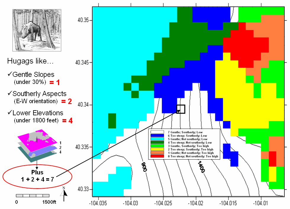
Figure
1.
Binary Progression Suitability map with combinations indicated.
A
further extension of the binary techniques uses a mathematical trick. The criteria maps are reclassified to a
binary progression of numbers (1, 2 and 4) instead of all 1’s for acceptable
habitat (figure 1). When these maps are
summed the result is a unique value for each combination of values. For example, a location with a sum of 3 can
only occur if it is gently sloped (1) plus southerly exposed (2) plus too high
(0). The best habitat is indicated by
the value 7 (1+2+4= 7).
A Binary Progression Suitability map
contains a great deal of information beyond that of a simple binary or ranking
map as it indicates the actual combinations of acceptable and unacceptable
conditions. If there are more than three
criteria layers, the progression is just extended (…8, 16, 32, 64, etc.). In all cases the permutations result in a
unique sum.
However
all binary models suffer the same problem—things are either good or bad with no
degree of goodness. It’s like pass/not
pass grading that doesn’t distinguish exceptional performance (either good or
bad) and forces a sharp boundary instead of a gradient of performance.
Figure
2.
Average Suitability map with an average score for each
location.
Figure 2
depicts an alternative procedure where each of criteria layers are “graded” on
a scale from 1= very bad to 9= very good.
For this example the calibration was—
Slope Map: >40%= 1 (very bad);
30-40= 3; 20-30= 5; 10-20= 7; 0-10= 9 (very good)
Aspect Map: N, NE, NW= 1 (very bad);
E, Flat= 5; W= 6; SE, S, SW= 9 (very good)
Elevation Map: >1800ft= 1 (very
bad); 1400-1800= 3; 1250-1400= 5; 900-1250= 7; 0-900= 9 (very good)
…then
the individual criteria maps are averaged for an overall score. In addition, lakes are masked as they
represent impossible habitat (drowned Hugags).
The
result is an Average Suitability map containing
an overall score for each map location.
Note the results for the example location in both figure 1 and 2. The Binary Progression solution ranks it as
totally acceptable (7= gentle, southerly, low), while the Average Suitability
solution rates it as mediocre habitat (5.3= mid-range on a 1 to 9 scale). The dark green locations, on the other hand,
identify very good habitat (8-9 rating) and the bright red locations indicate
the worst habitat (1-2 rating).
The
continuous gradient solution provides significantly more information than any
of the binary techniques. In practice,
the individual map layers are assigned weights to indicate their relative
importance and a weighted-average is computed.
The areas with high scores can be isolated and designated sensitive
habitat areas for natural resource planning.
Figure
3.
Draping the Average Suitability map over the Elevation surface shows
good alignment with critical terrain features.
Figure 3
shows the average suitability model applied to a larger area based on freely
available 30m digital elevation data.
When the suitability map is draped on the terrain surface its results
are easily evaluated. The best areas
(dark green) align with the gentle, southerly sloped and relatively low
areas. The worst areas (bright red)
align with steep northerly sloped and relatively high areas.
In practical
applications, habitat modeling considers many more factors than simply terrain
configuration. For example, the model
could be extended to evaluate the additional criterion that “Hugags would prefer to be within or near forested areas”
(proximity to
Keep in mind that suitability modeling isn’t restricted to wildlife habitat analysis. The approach is just as valid for identifying “customer habitat” in geo-business, or crop suitability in agriculture, or pipeline suitability for identifying the best route. Like statistics, the suitability modeling cuts a wide swath through many applications as a fundamental analytical tool.
Logic and Extent Elevate
Suitability Models to New Levels
(GeoWorld, October 2004, pg. 20-21)
The previous sections on suitability modeling used wildlife habitat mapping to illustrate the development of progressively more powerful modeling approaches—binary, ranking, permutation and rating models. All four approaches used the same set of basic criteria—Hugag preference for gentle slopes, southerly aspects and lower elevations—as depicted in figure 1. The difference in how the processing takes place was the focus of discussion.
In the case of a binary model each consideration is treated as either good or bad and results in a habitat map that identifies just good and bad habitat areas. A ranking model, on the other hand, uses the same good/bad criteria but identifies the number of good factors for each map location with higher values indicating increasingly higher habitat ranking. A permutation model provides even more information by identifying the unique combination of good and bad factors occurring at each location.
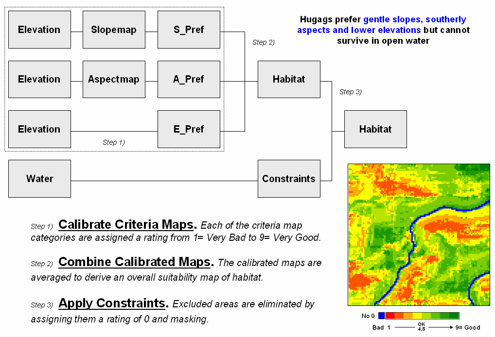
Figure 1. Model logic for basic Hugag habitat
suitability mapping.
A rating model is the most powerful approach. It breaks the good/bad dichotomy into a gradient of preference most often expressed as 1= very bad to 9= very good. For example, the preference for gentle slopes (S_Pref in figure 1) was assigned as 1 (very bad) = >40%; 3= 30-40; 5= 20-30; 7= 10-20; and 9 (very good) = 0-10%. In a similar manner, categories for aspect and elevation are calibrated then averaged and masked for constrained areas to generate the overall suitability map shown in the figure. This result contains continuous habitat values—considerably more information than simply the spatial coincidence of discrete areas of good/bad classifications.
While processing approach is an important consideration, the model logic and extent can be even more important in determining model accuracy. In practical applications, the habitat model would likely consider many more factors than simply terrain configuration. Figure 2 shows a flowchart of the extended model logic to evaluate the additional criteria that “Hugags would prefer to be in forested areas” (Forest map), that “Hugags would prefer to be near water” (proximity to Water map) and that “Hugags would prefer to be far from roads” (proximity to Roads map).
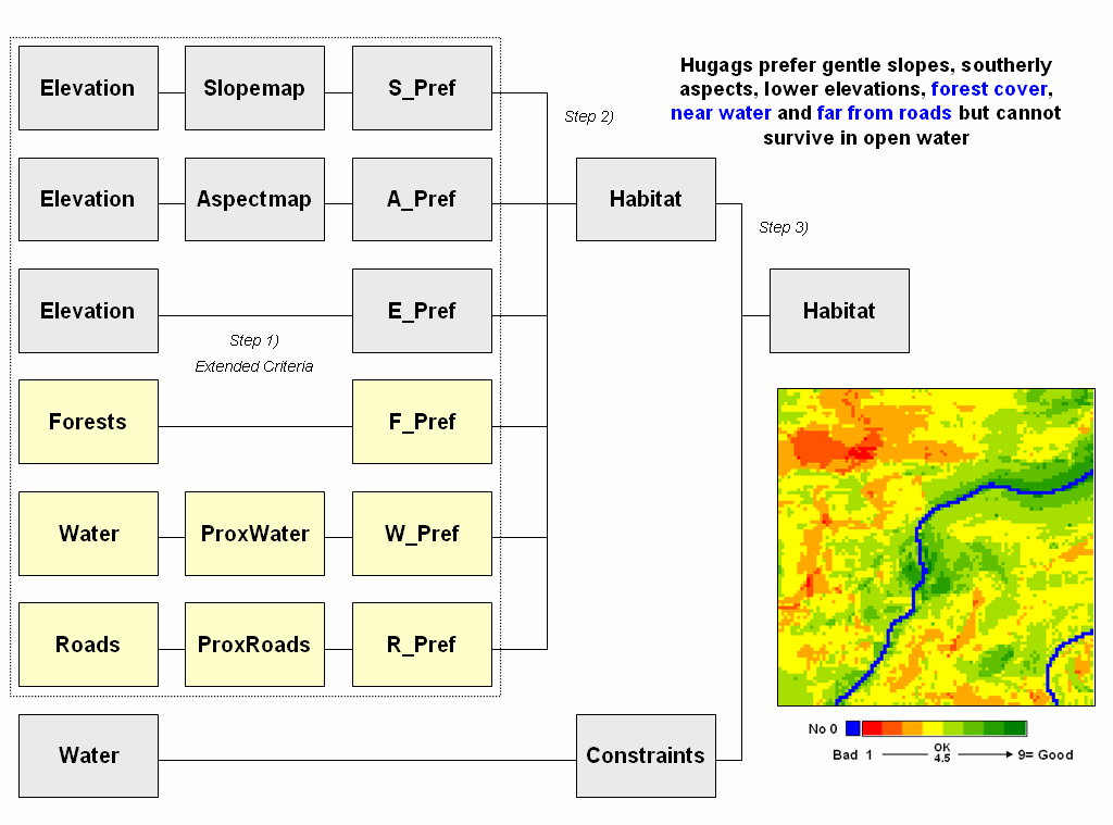
Figure 2. Extended model logic for considering Hugag
preference for being in forests, near water and far from roads.
In suitability modeling, these considerations are treated as separate sub-models to derive the necessary criteria, then calibrated on the 1 to 9 preference scale and averaged with the basic set of terrain considerations for an overall habitat map shown in the figure.
Note that a large part of the model’s strength or weakness is established in Step 1—calibrate criteria maps. As much as possible, the identification of map criteria needs to reflect good science and/or expert opinion to capture factors that are both important and easily measurable. Similarly, the calibration of the maps into the 1-9 preference range needs to capture realistic relative values, not whimsical or biased assignments.
Step2— combine
calibrated maps is another area requiring considerable understanding of the
system being modeled. A simple average
of the calibrated map layers assumes that all of the criteria are equally
important. The right inset in Figure 3
shows the habitat results for expert thinking that Hugags are “10 times more concerned about slope, forest and water
considerations than they are about aspect, elevation and roads
considerations.”
The procedure for determining relative importance involves computing the weighted-average of the six map layers. It is analogous to a professor’s grading some exams more important than others in determining a class grade. In this case, the map values correspond to student grades on each exam; each student is represented as a grid cell on the map, kind of like their desk seats in the classroom floor plan.
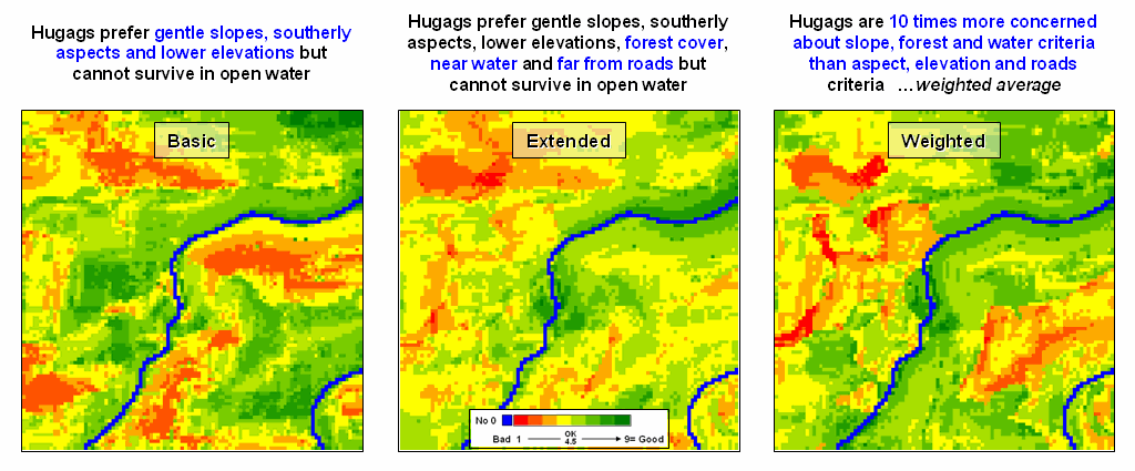
Figure 3.
Habitat rating maps for progressively more powerful model logic and
processing.
Note the
similarities and differences in the maps induced by the additional criteria
(Extended) and relative weighting of map layers (Weighted). Provided expert opinion is sound, the
weighted map on the right would be considered the most accurate representation
of Hugag habitat.
Keep in mind that calibrating and weighting are extremely critical steps in suitability modeling. Procedures, such as Delphi and AHP, can be used to derive these factors in a quantitative, objective, consistent and comprehensive manner (see Author’s Notes). In addition, purposeful changing these factors can reflect different assumption scenarios analogous to “what if” questions applied to traditional spreadsheet analysis.
From this perspective, it is how the suitability maps change
that becomes information about the sensitivity of a project area to the interplay
of criteria, calibrations and weights.
This takes us well beyond mapping to assessing the spatial relationships
within a system and their logical expression within a GIS. As GIS technology matures, the focus is
shifting from simply access of static map products depicting physical features
for navigation and inventory to a dynamic environment that enables “thinking
with a stack maps” within decision-making contexts.
Breaking Away from
Breakpoints
(GeoWorld, June 2011)
An earlier section in
this online book (“Determining Exactly Where
Is What,” Introduction)
discussed the differences between precision and accuracy. In short, Precision addresses the
exactness of the shape and positioning of spatial objects (the “Where”
component); whereas Accuracy addresses the correctness of the
characterization/classification of map locations (the “What” component).
Mapping
tends to focus on precision, while map analysis and modeling primarily are
concerned with accuracy. For example,
thematic mapping often assigns the average from a wealth of spatial samples
although the standard deviation is high.
The result is high precision in delineating a spatial object (e.g.,
district boundary) but very low accuracy due to the over generalization (e.g.,
average elevation) as discussed in an earlier column (“What’s
Missing in Mapping?” Topic 18).
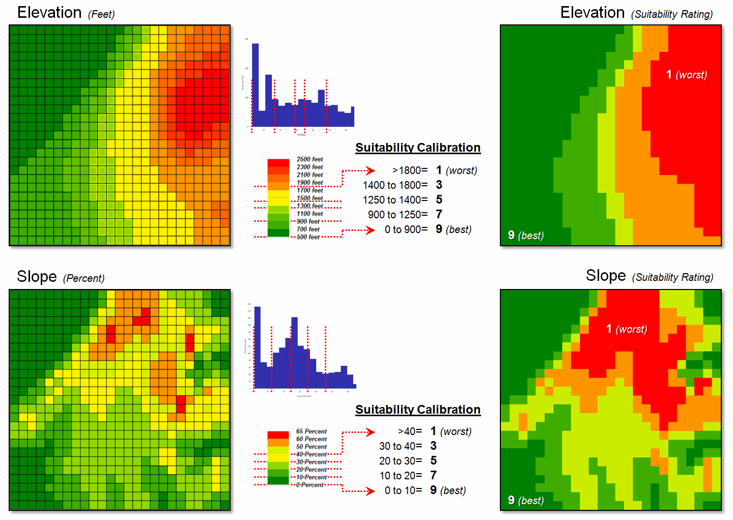
Figure 1. Abrupt breakpoints often
are used to calibrate suitability.
But
let’s consider a less obvious source of inaccuracy— broad categorization of
suitability model inputs. For example,
the previous sections described a simple “rating” habitat model with strong
animal preferences for terrain configuration: prefers low elevations
(severe nose bleeds at higher altitudes), prefers gentle slopes (fear of
falling over and unable to get up) and prefers southerly aspects (a
place in the sun).
Figure
1 depicts the calibration of the Elevation and Slope maps into a “graded
goodness scale” from 1= worst to 9= best in terms of relative habitat
suitability. Note the discrete ranges of
map values equated to the suitability ratings—that’s the way humans think. For example, all locations between 900 and
1250 feet are assigned the same 7.0 suitability value. But it seems common sense that an elevation
of 900 isn’t that different from 899, while it is substantially different from
1249. The relative differences are more
an artifact of the discrete steps than real habitat variations.
However,
both the ratings and the map values define continuous numerical scales that
even allow for decimal-level differences.
The left side of figure 2 shows the discrete breaks in suitability ratings
imposed by the step function approach.
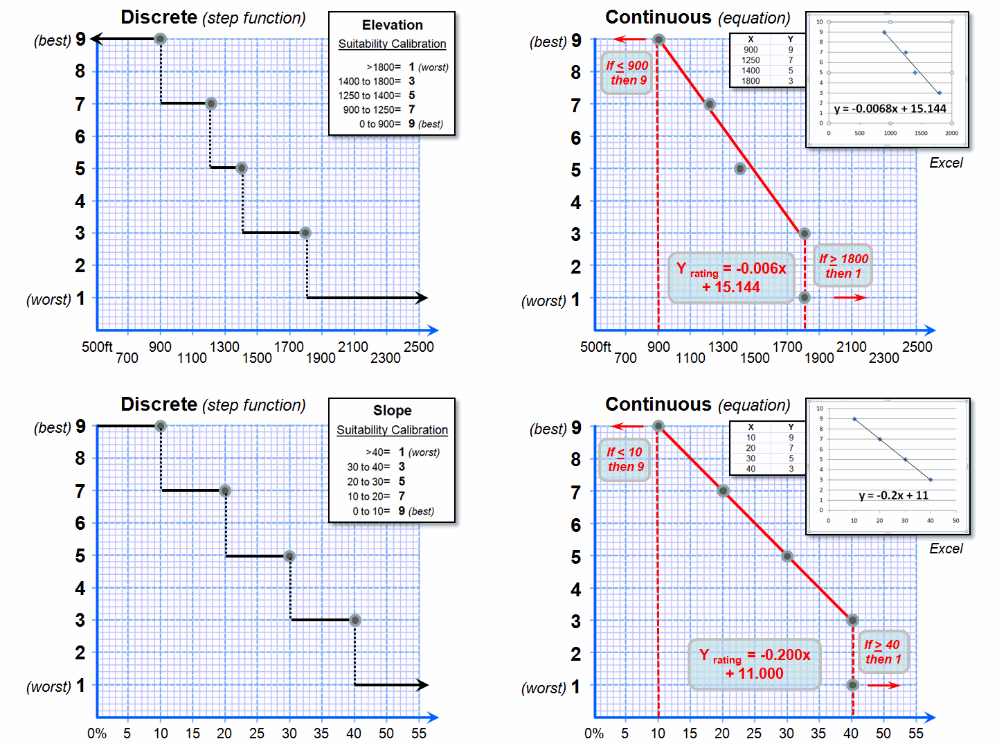
Figure 2. Curve-fitting can be used
to convert suitability step functions into continuous equations for increased
accuracy.
A
more robust approach develops a continuous relationship based on the same
calibration information. Excel can be
used to derive an equation (trend line) that calculates the suitability rating
associated with the full range of map values.
For example, a 950 foot elevation calculates to an 8.68 rating (Yrating= -.006Xelevation950 + 15.144=
8.68), whereas an elevation of 1200 calculates to 6.98.
Both
conditions would be assigned a rating of 7 under the step function approach—inaccuracy
induced by a comfortable but overly generalized categorization. The use of a continuous equation instead of
discrete reclassifying ranges has the effect of “smoothing” the ratings from
one point to the next for a gradient of suitability instead of a set of abrupt
breakpoints. The curve-fitting does not
have to be linear, with more accurate results (but uglier equations) derived
from exponential relationships.
Figure 3 compares the effects
of discrete and continuous suitability calibrations. Note the “pixilated appearance” of the
continuous suitability assignments (middle) over the sharp rating transitions
in the discrete assignments (left-side).
This more exacting information carries over to the suitability models
themselves (right-side). A difference
map between the model runs shows some locations with as much as 1.5 rating
difference—just by changing the approach.
Figure 3. More accurate suitability
ratings from continuous equations can significantly affect modeling results.
But the more exacting characterization
only works for quantitative mapped data like elevation and slope. Qualitative maps (categorical data) are stuck
with sharp boundaries in both geographic and numeric space. Aspect is even more interesting as it is
continuous in geographic space but discontinuous in numeric space as it wraps
around on itself (1 and 359 degrees are more alike than 1 and 90 degrees).
The bottom line is that
good GIS modelers view maps as “numbers first, pictures later” with the both
the spatial and numerical character of mapped data determining appropriate
procedures and the level of precision and accuracy in model results.
_____________________________
Author’s Note: While
there are several curve-fitting programs on the Internet, Excel is generally
available and provides for both linear and exponential equations. To identify the fitted
equation…
1) create two data columns
(X= map value and Y= rating),
2) highlight the columns and click on the Insert
tabà Scatter Chart to create a plot,
3) click on the plot and select the Layout Tabà Trendline and specify Linear or Exponential,
4) right-click on the Trendline and select Format
Trendline, and
5) click the “Display Equation on chart” box.
Extended Experience Materials
Extended
Experience Materials: see www.innovativegis.com/basis/,
select “Column Supplements” for a PowerPoint slide set, instructions and free
evaluation software for classroom or individual “hands-on” experience in
suitability modeling. If you are viewing
this topic online, click on the links below:
- Suitability Modeling Slide Set
– a series of PowerPoint slides describing Binary, Ranking and Rating
approaches to suitability modeling described in GeoWorld, July and August,
2004 Beyond Mapping columns. (627KB).
- For hands-on
experience in Suitability Modeling—
- <click here> to download and
install a free version of MapCalc
Learner software for self-learning and classroom use.
- <click
here> to download the Hugag database, Hugag script
and Hugag.ppt self-extracting
file; extract the files to the data folder for the newly installed MapvCalc Learner software— C:\Program
Files\Red Hen Systems\MapCalc\MapCalc Data\.
- Click Startà Programsà MapCalc Learnerà
MapCalc Learner to access the MapCalc Software. Select the Hugags.rgs database you downloaded.
 Click on the Map Analysis button to pop-up the script
editor. Select Scriptà Open and select the Hugag.scr file you downloaded. A series of commands comprising the
model will appear.
Click on the Map Analysis button to pop-up the script
editor. Select Scriptà Open and select the Hugag.scr file you downloaded. A series of commands comprising the
model will appear.- Double-click on the first command line Slope Elevation
Fitted for Slopemap note the dialog box specifications,
and press OK to submit the command.
 Minimize the script window and use the
map display/navigation buttons in the lower toolbar to explore the output
map.
Minimize the script window and use the
map display/navigation buttons in the lower toolbar to explore the output
map.
See http://www.innovativegis.com/basis/Senarios/Movies/MC_Basics.exe (click “Open”) for a short online video of demonstrating several of the MapCalc display functions.- Repeat the process in sequence using the other command lines while
relating the results to the discussion in this topic and the slide set
identified above.
…direct questions
and comments to jberry@innovativegis.com.
…an additional set of tutorials using MapCalc software is
available online at…
http://www.innovativegis.com/basis/Senarios/Tutorials/Default.htm
…example techniques
and applications using map analysis are available online at…
http://www.innovativegis.com/basis/Senarios/Default.html