Applying MapCalc Map Analysis Software
Identifying Campground Suitability: A recreation specialist needs to generate
a map that identifies the relative suitability for locating a campground. In an initial planning session it was
determined that the best locations for the campground is on gently sloping
terrain, near existing roads, near flowing water, with good views of surface
water and oriented toward the west.
<click here>
for a printer friendly version (.pdf)
Processing Flow.
 Campground
Suitability—Model Logic
Campground
Suitability—Model Logic
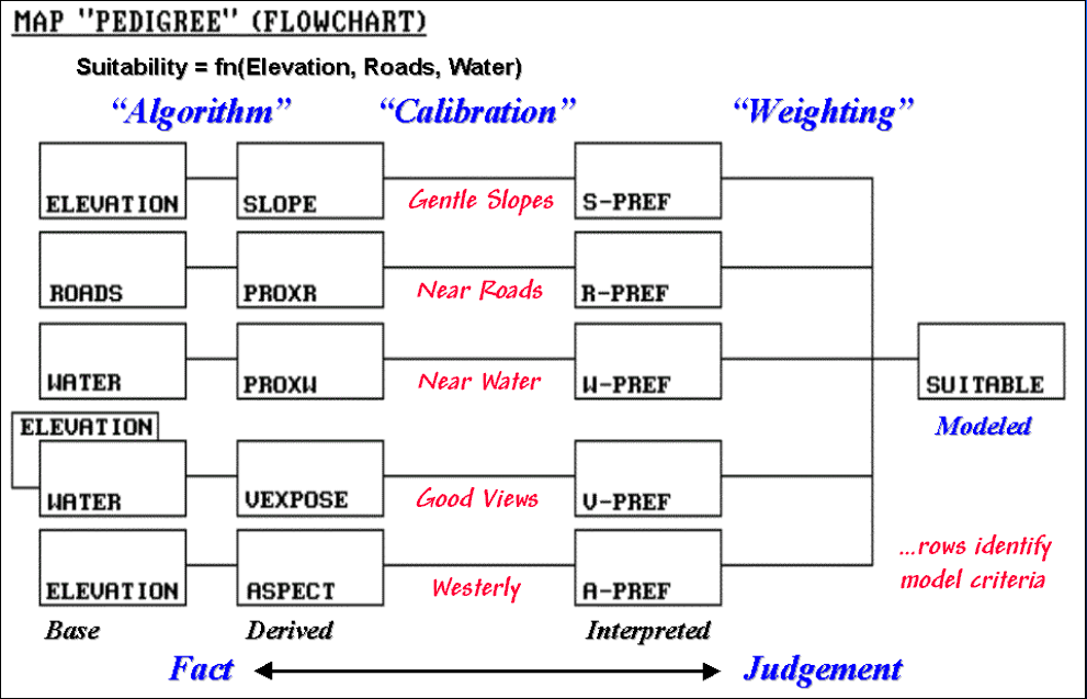
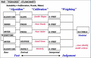
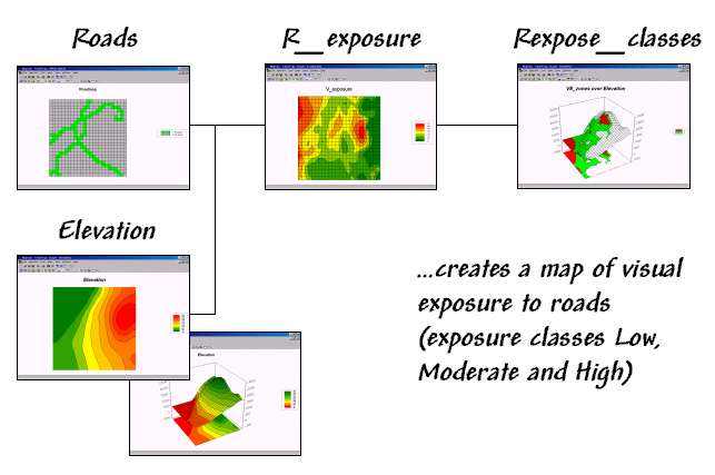
All GIS models can be
expressed as a flowchart of processing steps.
In this example, SLOPE is derived from a base map of ELEVATION. In turn, the SLOPE map is interpreted for
areas of “relative goodness” in terms of terrain steepness and stored as the
S_PREF map.
The each row in the flowchart is evaluated to reflect preferences for locating a campground—
gentle slopes l near roads l near water l good views of water l and westerly oriented.
The final step combines the maps of the five criteria for a map of the overall suitability (SUITABLE). Note that the columns in the flowchart reflect increasing abstraction from Base maps of physical features, to Derived maps of spatial context, to Interpreted maps of relative goodness, and finally to a Modeled map of suitability. The movement from maps of physical Fact to decision Judgment involves a logical sequencing of map analysis operations.
You can take a “guided tour” of this model using the MapCalc Learner software…
Accessing a MapCalc Database
To begin a MapCalc session—
- Click on the Windows Start button.
- Navigate to Programs à Red Hen Systems à MapCalc and click on the MapCalc icon.
- Choose Open existing map set from the MapCalc Quick Start menu and open the Tutor25.rgs database. The database will be accessed, several of the base maps will be opened and a 2-D display of the Elevation map will be maximized.
Accessing a Stored Script
Now open the command macro for Campground Suitability—
- Access
the Grid Analysis module by pressing the Grid Analysis button on
the Main Toolbar

- Select Scriptà Open from the Map Analysis menu
- Navigate to the C:\Program Files\Red Hen Systems\MapCalc\MapCalc Data\Scripts folder open the Campground.scr script
 Script
Procedures
Script
Procedures
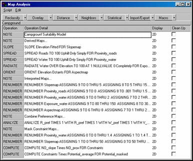
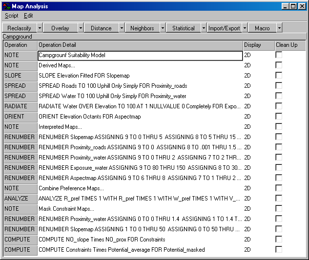
Each line of the script contains an individual MapCalc command. The command lines are executed in their listed order (top to bottom). You can view a command’s specifications by double-clicking on a command line, then click “OK” to execute the command and display the derived map. In many instances the default map displays are modified for the ones shown below using the procedures described in Tutorial Lessons 1 through 6.
Base Maps. The Base Maps needed include:
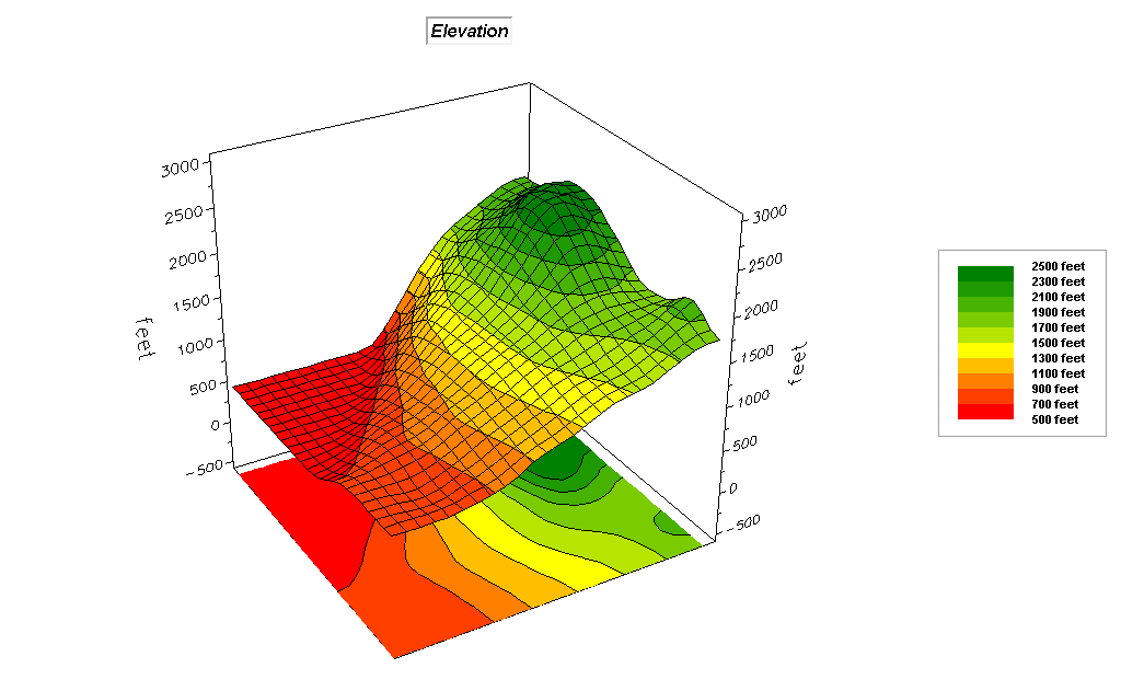 Elevation Map. Each grid cell value identifies its elevation
forming a continuous terrain gradient.
Elevation Map. Each grid cell value identifies its elevation
forming a continuous terrain gradient.
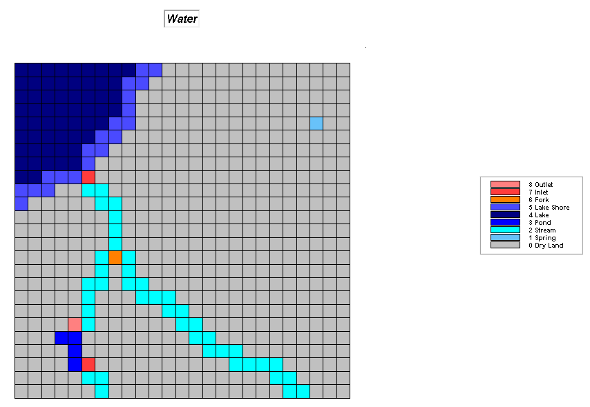 Water Map. Each grid cell value identifies surface water
present.
Water Map. Each grid cell value identifies surface water
present.
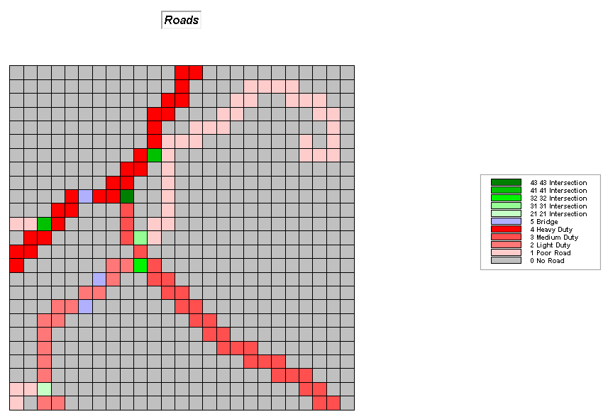 Roads Map. Each grid cell value identifies the type of
road present.
Roads Map. Each grid cell value identifies the type of
road present.
Step 1, Derived Maps.
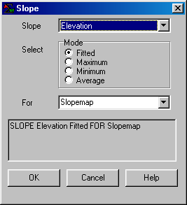
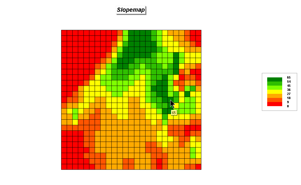 Slopemap.
The terrain steepness varies from 0% to 65% slope.
Slopemap.
The terrain steepness varies from 0% to 65% slope.

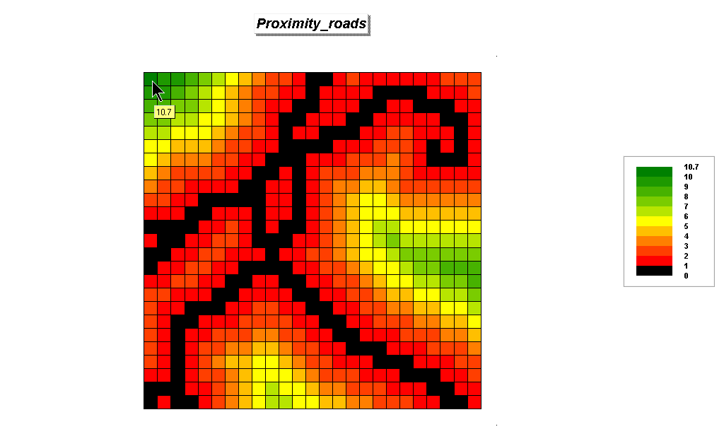 Proximity_roads. The distance from roads varies from 0 (road
present) to 10.7 cells away. Since each
cell is 100 meters (328 feet), the farthest location in the northeast corner is
1.07 kilometers (10.7*328=3509.6/5280= .665 miles) away from the nearest road
location. For this display, the “Shading
Manager” was set to Equal Ranges, number of ranges to 11, black assigned to
range 0-1, red to range 1-2, yellow to range 5-6 and green to range 10-10.7.
Proximity_roads. The distance from roads varies from 0 (road
present) to 10.7 cells away. Since each
cell is 100 meters (328 feet), the farthest location in the northeast corner is
1.07 kilometers (10.7*328=3509.6/5280= .665 miles) away from the nearest road
location. For this display, the “Shading
Manager” was set to Equal Ranges, number of ranges to 11, black assigned to
range 0-1, red to range 1-2, yellow to range 5-6 and green to range 10-10.7.
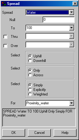
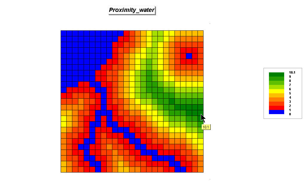 Proximity_water. The distance from water varies from 0 (water
present) to 10.1 cells away. For more
information on how distance is measured, see “Determining Proximity”
application scenario.
Proximity_water. The distance from water varies from 0 (water
present) to 10.1 cells away. For more
information on how distance is measured, see “Determining Proximity”
application scenario.
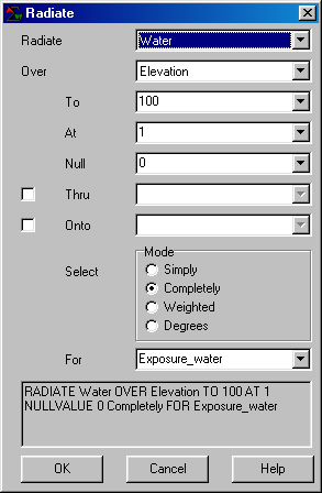
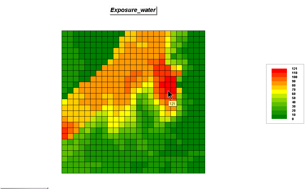 Exposure_water. The relative exposure to water varies from 0
(not seen) to 121 water cells seen from the location indicated in the
figure. Since there is 128 cells with
water present (blue area in the Proximity_water map above), a location that is
visually connected to 121 cells “sees” a lot of water (121.128= 95% of the
water area). For more information on how
visual exposure is measured, see “Determining Visual Exposure” application
scenario.
Exposure_water. The relative exposure to water varies from 0
(not seen) to 121 water cells seen from the location indicated in the
figure. Since there is 128 cells with
water present (blue area in the Proximity_water map above), a location that is
visually connected to 121 cells “sees” a lot of water (121.128= 95% of the
water area). For more information on how
visual exposure is measured, see “Determining Visual Exposure” application
scenario.
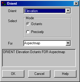
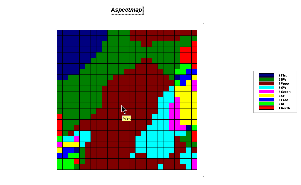 Aspectmap. The dominant terrain orientation is West (7=
West) and Northwest (8= NW). The large
flat area (no aspect) in the upper left corner is a lake (blue area in the
Proximity_water map above).
Aspectmap. The dominant terrain orientation is West (7=
West) and Northwest (8= NW). The large
flat area (no aspect) in the upper left corner is a lake (blue area in the
Proximity_water map above).
Step 2, Interpreted Maps.

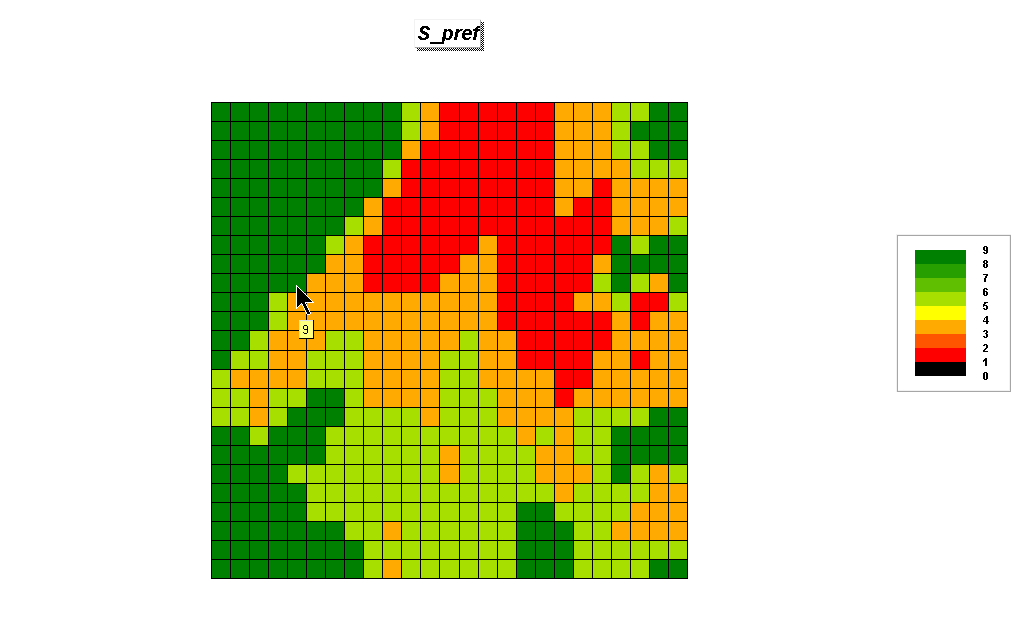 S_pref. The “Slopemap” is calibrated to a 1 (worst)
to 9 (excellent) scale of campground suitability with gently sloped areas rated
the best (green tones).
S_pref. The “Slopemap” is calibrated to a 1 (worst)
to 9 (excellent) scale of campground suitability with gently sloped areas rated
the best (green tones).
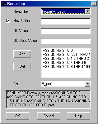
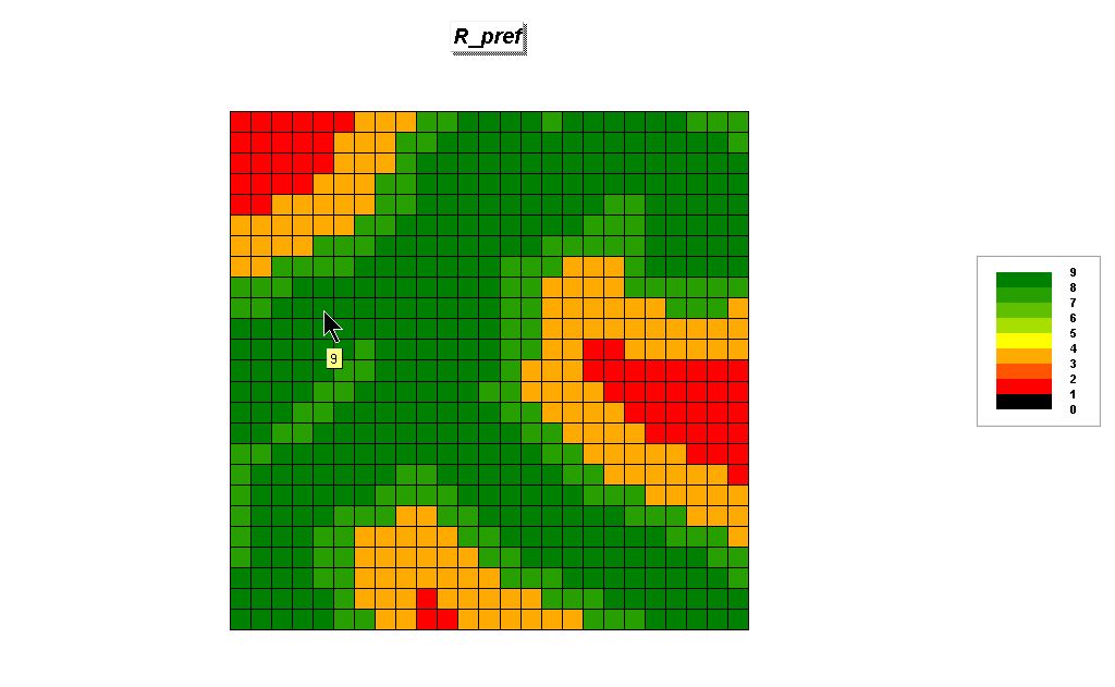 R_pref.
The “Road_proximity” map
is calibrated to a 1 (worst) to 9 (excellent) scale of campground
suitability with areas close to a road rated the best (green tones).
R_pref.
The “Road_proximity” map
is calibrated to a 1 (worst) to 9 (excellent) scale of campground
suitability with areas close to a road rated the best (green tones).
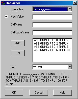
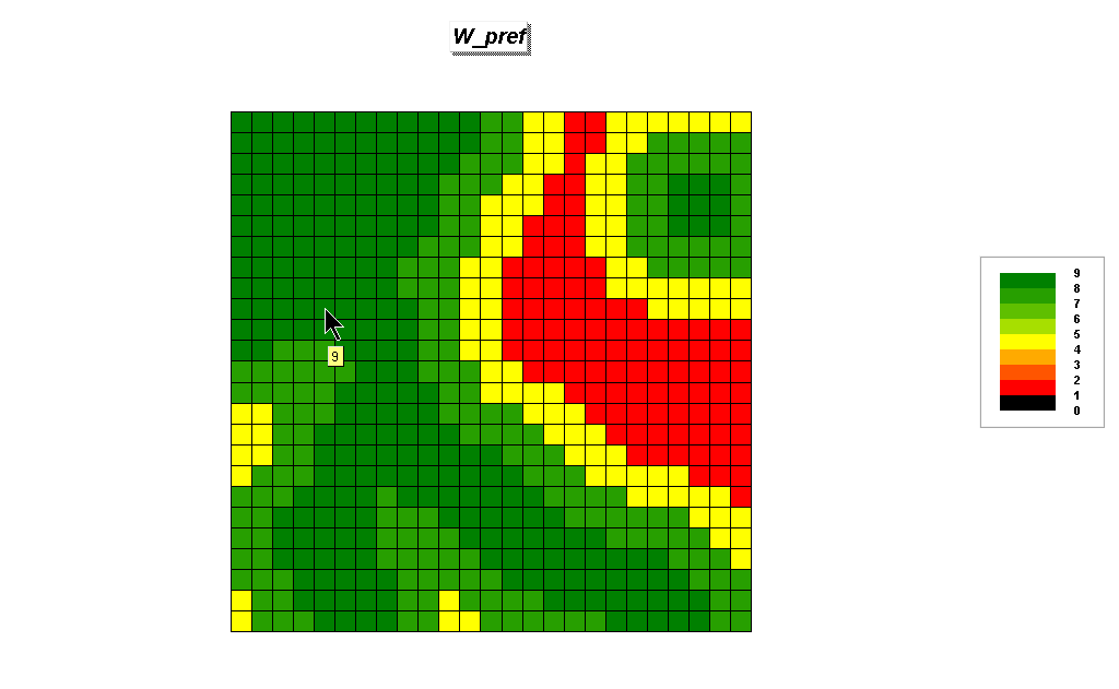 W_pref.
The “Water_proximity” map
is calibrated to a 1 (worst) to 9 (excellent) scale of campground
suitability with areas close to water rated the best (green tones).
W_pref.
The “Water_proximity” map
is calibrated to a 1 (worst) to 9 (excellent) scale of campground
suitability with areas close to water rated the best (green tones).
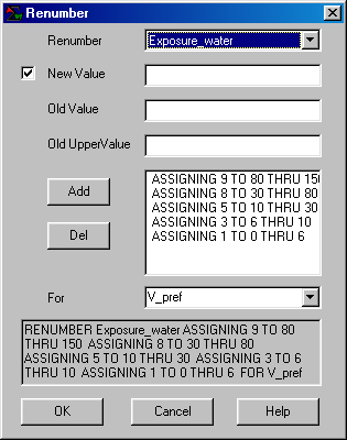
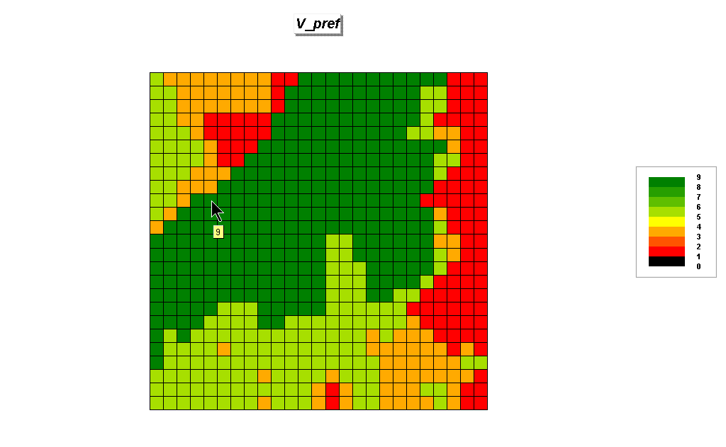 V_pref.
The “Exposure_water” map
is calibrated to a 1 (worst) to 9 (excellent) scale of campground
suitability with areas “seeing” a lot of water rated the best (green tones).
V_pref.
The “Exposure_water” map
is calibrated to a 1 (worst) to 9 (excellent) scale of campground
suitability with areas “seeing” a lot of water rated the best (green tones).
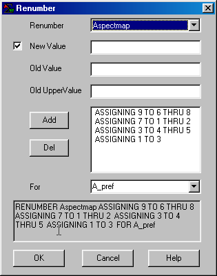
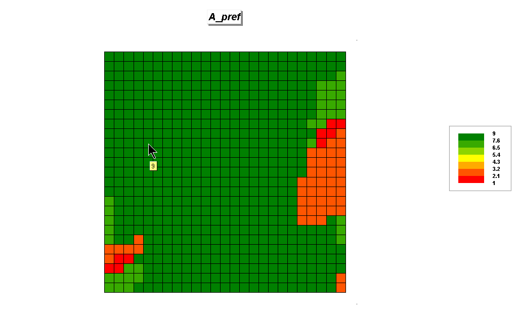 A_pref.
The “Aspectmap” is calibrated to a 1 (worst) to 9 (excellent)
scale of campground suitability with westerly oriented terrain rated the best
(greentones).
A_pref.
The “Aspectmap” is calibrated to a 1 (worst) to 9 (excellent)
scale of campground suitability with westerly oriented terrain rated the best
(greentones).
Step 3, Combine Preference Maps.
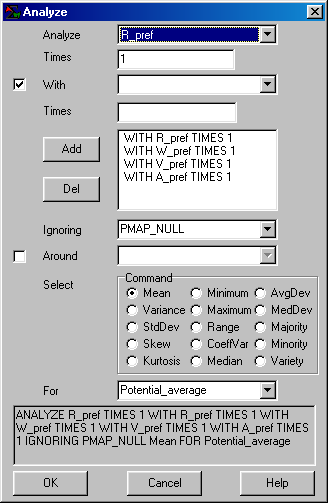
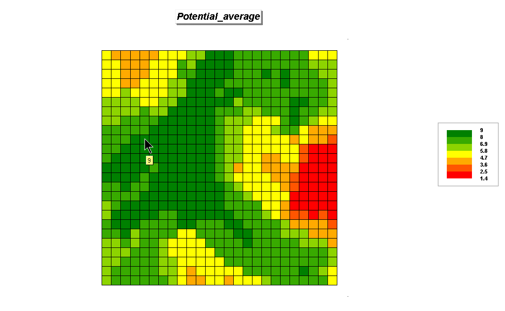 Potential_average. An overall suitability map is generated by
calculating the average of the individual preference maps. Areas with higher average suitability (green
tones) are the best areas “overall.”
Potential_average. An overall suitability map is generated by
calculating the average of the individual preference maps. Areas with higher average suitability (green
tones) are the best areas “overall.”
Step 4, Mask Constraint Maps.
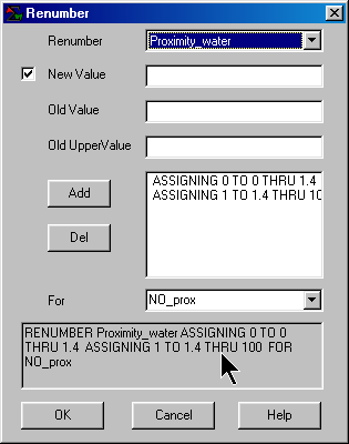
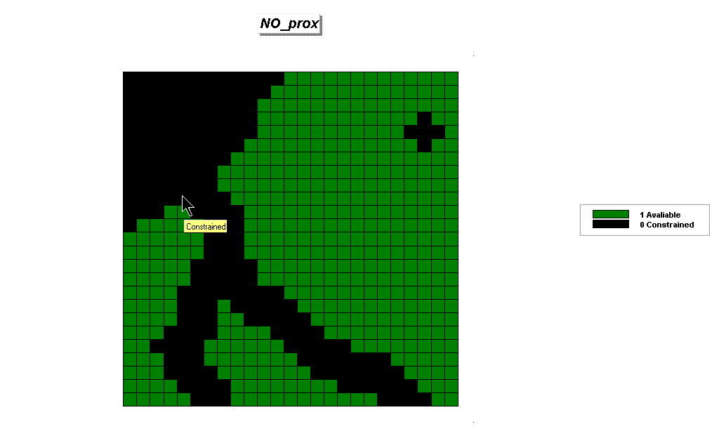 No_prox. Areas too close to water (0 to 1.4 cells)
are legally constrained and are not available for locating a campground (black
areas).
No_prox. Areas too close to water (0 to 1.4 cells)
are legally constrained and are not available for locating a campground (black
areas).
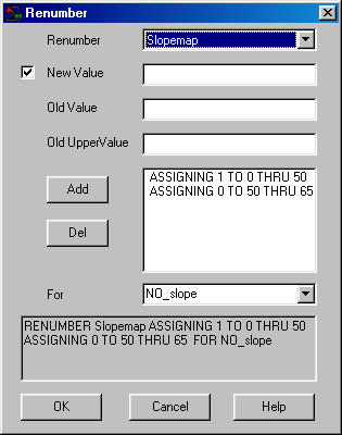
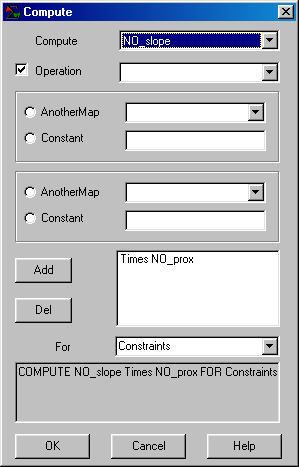
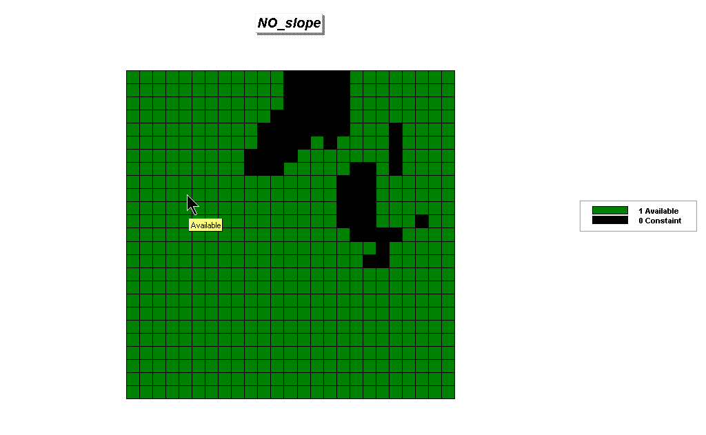 No_slope. Areas steep (greater than 50% slope) are
legally constrained and are not available for locating a campground (black
areas).
No_slope. Areas steep (greater than 50% slope) are
legally constrained and are not available for locating a campground (black
areas).
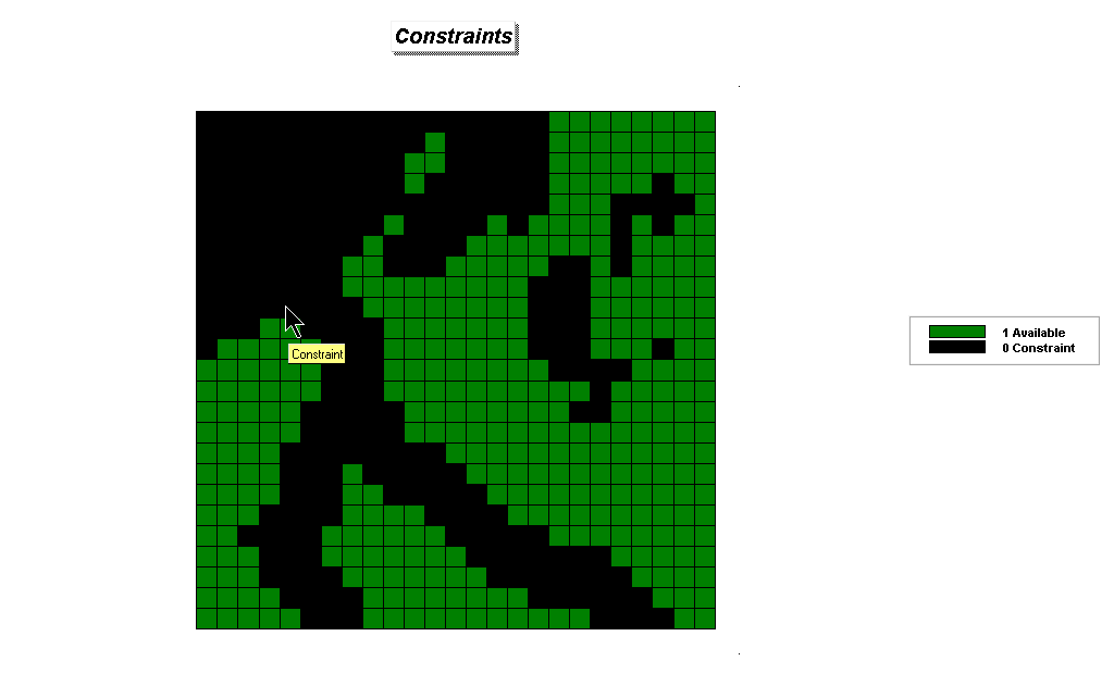 Constraints. The two individual constraint maps are
multiplied together for an overall map of constraints (black areas)— 0*1, 1* 0
or 0*0. Only areas that are available on
both maps are identified as available overall— 1*1.
Constraints. The two individual constraint maps are
multiplied together for an overall map of constraints (black areas)— 0*1, 1* 0
or 0*0. Only areas that are available on
both maps are identified as available overall— 1*1.
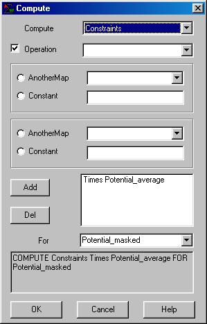
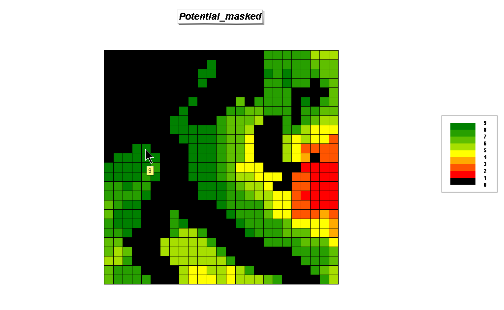 Potential_masked. The same binary masking procedure is used by
multiplying the “Constraints” map by the “Potential_average” map. The result is a map with 0 indicating
unavailable areas and higher values indicting the best areas.
Potential_masked. The same binary masking procedure is used by
multiplying the “Constraints” map by the “Potential_average” map. The result is a map with 0 indicating
unavailable areas and higher values indicting the best areas.
Summary. The simple Campground Suitability model identifies the “relative goodness” of each map location for a campground. This suitability map can be used to narrow field work and serve as a starting palace for further map analysis. The model can be extended in two ways. The logic can be enhanced to include other factors, such as “being in or near forested areas” as best…
SPREAD Forests TO 100 Uphill Only Simply FOR Forest_prox
RENUMBER Forest_prox ASSIGNING 9 TO 0 ASSIGNING 7 TO 1 THRU 2 ASSIGNING 3 TO 1.01 THRU 4 ASSIGNING 1 TO 4 THRU 100 FOR F_pref
Also, the model’s parameters and weights can be changed to reflect different interpretations, such as proximity to water more important than terrain steepness…
ANALYZE S_pref TIMES 1 WITH R_pref TIMES 10 WITH W_pref
TIMES 5 WITH V_pref TIMES 5 WITH A_pref TIMES 5 WITH F_pref TIMES 5 IGNORING
PMAP_NULL Mean FOR Potential_average2
COMPUTE Constraints Times Potential_average2 FOR
Potential_masked2
Give the extensions a try on your own. You can compare the two results by…
COMPUTE Potential_masked Minus Potential_masked2 FOR Difference
…areas with 0 assigned indicate no change; sign of the values indicate type of change (positive means original rating higher); and magnitude of the value indicates the amount of change (large values indicate a lot of change).