|
The Precision Farming Primer |
|
|
|

Part 1. Yield Mapping
Considerations
Yield Mapping Sparks Precision
Farming Success by Neil Havermale — discusses several factors affecting spatial accuracy
in yield mapping
Yield Monitors Create On- and
Off-Farm Profit Opportunities by Tom Doerge — discusses the benefits of yield monitoring and mapping
Part 2. Investigating Interpolation Results
Comparing Interpolated and
Extrapolated Data — investigates the relative
performance of spatial interpolation and extrapolation
Normalized
Map Comparisons — compares raw and normalized maps
Defining
the Norm — describes a procedure for
normalizing mapped data
Comparing
the Comparable — discusses the importance of
comparing normalized maps
Visually Comparing Normalized
Residual Maps — visually compares normalized maps
of Average, IDW, Kriging and MinCurve interpolation results
More
on Zones and Surfaces — discusses the relative variation "explained" by
zone and surface maps
Last Word on Zones and Surfaces — discusses the effects of "unexplained" variation
in site-specific management
Excel Worksheet Investigating
Zones and Surfaces —
provides access to Excel worksheets used in the zone and surface discussions
Part 3. More on Spatial Dependency
Spatial Dependency and Distance — describes a procedure for relating spatial dependency
and distance
Mapping
Spatial Dependency —describes
a procedure for mapping localized spatial dependency
Excel Worksheets Investigating
Spatial Dependency —
provides access to Excel worksheets used in the spatial dependency discussions
Part 4. More on
Correlation and Comparing Maps
Excel Worksheet Investigating Map
Correlation and Prediction — worksheet
containing the calculations for determining map correlation and predictive
modeling
Validity of Statistical Tests
with Mapped Data by William Huber — discusses concerns in applying
traditional non-spatial techniques to analyze mapped data (in prep)
Excel Worksheet Investigating
Map Surface Comparison — worksheet containing the calculations for t-test, percent
difference and surface configuration examples
(Back to the Table of Contents)
______________________________
Part 1. Yield Mapping Considerations
Yield Mapping Sparks Precision Farming Success (return to top of Appendix A)
By Neil Havermale
Farmers Software Association, 800
Stockton Ave., Fort Collins, CO 80524. Published as part of "Who's Minding the
Farm" article on Precision Farming in GIS World, February 1998, Vol. 11,
No. 2, pg. 50.
The GIS-based crop yield data layer is the
most important enabling element in the precision farming revolution. An
accurate yield map integrates nature's climatic effects and a farmer's
management decisions. A yield map can identify natural and manmade
variations in a farmed landscape, a crop's genetic expression in a particular
season's environment and more.
There are four general sources of bias in
most "as recorded" yield data sets: antenna placement, GPS latency,
instrumentation and modeling errors. Because actual yield is the basis of
future prescriptive action in a site-specific farming system, spatial accuracy¾when tied to a proper model of a computer's threshing action¾determines the final quality of any prescriptive method.
Antenna Placement. In early applications, yield monitors were installed as retrofits on new or old combines. Accurately placing a GPS antenna on a combine's centerline is critical. With the increasing accuracy of differentially corrected GPS to within a meter, a foot or two of misplacement can result in the antenna offset bias pattern shown in figure A.1.
|
|
|
|
Fig. A.1. Accurately placing a GPS antenna on a combine's centerline is critical as illustrated by an example of uncorrected (left) and corrected antenna offset (right). |
|
GPS Latency. Latency in various GPS receivers' NMEA
navigation strings has proven to be less than "real time." In
fact, one of the early differentially corrected GPS systems widely integrated
into the leading yield monitor had as much as a 6-8 second latency. The
receiver's latency in this case was directly tied to the differential
correction of the raw pseudoranges.
Instrumentation Error. There are two groups of current sensors in the
GPS combine: mass deflection strain gauges and clean grain volume estimation
via infrared beams. A simple examination of the placement of either of
these designs in the combine will reveal that any slope in the field can easily
distort the geometry of the clean grain path of travel. None of the
current yield monitors provide a sensor or correction for instrumentation
failure due to slope.
Model Deconvolution. The modern combine is a marvel. It can
digest literally tons of biomass in an hour, sorting that biomass into clean
grain measured by a grain flow sensor. Material other than grain goes out
the back as chaff. When properly adjusted and operated, the loss of grain
out the back with the chaff will be less than 1 percent. A combine is a
lot like a lawn mower. It can stall if pushed too quickly into tall,
heavy and wet grass; so its general design has important features that buffer
this effect.
Site-specific farming isn't a new idea. It's as old as childhood stories of Indians showing pilgrims how to plant corn with a fish as a source of fertility. The promise of modern GIS applications tied to GPS offers users the ability to gain micromanagment of farming practices, maybe not to a single plant like the pilgrims, but certainly to 1/100th of an acre. Precision farming systems literally represent a growing opportunity.
Yield Monitors Create On-
and Off-Farm Profit Opportunities (return to top of Appendix A)
By Tom Doerge
Pioneer H-Bred International, Crop Management, Research & Technology, P.O
Box 1150, Johnston, Iwoa, 50131. Published in Crop Insights, 1999,
Vol. 9, No. 14, Pioneer Hi-Bred International, Inc., Johnston, Iowa.
Summary
- Adoption rates of yield monitoring and variable-rate technologies within the Corn Belt of North America are currently no higher than 13% but are projected to increase several fold in the next 3-5 years.
- The advantages of variable-rate input applications are generally limited to in-field benefits such as reduced input costs and/or increased marketable yields.
- In contrast, yield monitoring and mapping offer many other on-farm benefits including real-time information during harvest, easier on-farm testing, better variable-rate management, evaluation of whole-field improvements, and creation of a historical spatial data base.
- Additional off-farm benefits of yield monitoring include more equitable landlord negotiations, crop documentation for identity preserved marketing, "traceback" records for food safety, and documentation of environmental compliance.
- Growers who will profit most from yield monitor use are those needing help keeping detailed field-by-field records, those not deterred by the "yield monitor learning curve", and those willing to effectively use additional sources of spatial data.
Each year, an increasing number of growers are adopting precision farming practices to gain efficiency and improve management of their operations. The two primary precision practices used in the Corn Belt of North America are yield monitoring and variable-rate application of crop inputs.
Recent surveys indicate that about 10 to 13 % of farmers in the Corn Belt region own yield monitors and a similar percentage own or use some form of variable-rate input application equipment (Khanna, 1998; Marks, 1998). These surveys also point out that the main barriers to adoption of these technologies are the high costs of equipment and training, and uncertainty about returns to the farm (Wiebold et al., 1998).
Frequently, growers or their bankers express reluctance in purchasing or financing a yield monitor because they can’t "pencil out" the immediate return for their operation. This Crop Insights will examine how profitability of the two major precision farming tools can be evaluated.
Measuring Profitability in Precision Farming
When comparing the profit opportunities of the two major precision farming tools, variable-rate is much easier to quantify than yield monitoring/mapping. In spite of this, yield monitoring and mapping is likely to be the more widely adopted and profitable tool in the future. By providing new information for improved site-specific and whole-farm management, yield monitoring and mapping allows farmers to be better managers of their operations. But this process is necessarily long-term, and placing an immediate value on it is not always possible.
Variable-Rate Inputs
The costs and benefits of a variable-rate input strategy are easily measured in controlled field experiments, so the profitability of these practices can be directly calculated.
|
|
Variable-rate application of plant nutrients, for example, is most profitable with high-yielding and high-value crops, where the soil level of the nutrient being applied is highly variable, and where there is a strong expectation of increasing yields in areas of the field that would otherwise be underfertilized.
The advantages of variable-rate application of crop inputs are generally limited to in-field benefits such as reduced input costs or increased marketable yields. Some of the site-characterization data used in developing variable-rate input strategies can be used in future seasons, although re-sampling of dynamic site features such as soil nutrient levels and pest infestations is often required.
Yield Monitoring and Mapping
In contrast to variable-rate input strategies, yield monitoring and mapping allows growers to view their overall management system from a more "whole-farm" perspective (Olson, 1998). Once yield monitoring is initiated, growers realize that fields can be highly variable, and often seize the opportunity to tailor their management in a much more site-specific manner.
|
|
|


Finally, growers can use yield maps as a feedback tool or "report card" to help monitor the performance of specific management inputs and decisions. In short, yield monitoring can change the perspective of producers as they learn to appreciate the value of detailed yield information and then strive for more data-driven optimization and risk management in their operations.
Unfortunately, this "holistic" benefit of yield monitoring can be hard to measure. In addition, there are several specific reasons why it is difficult to precisely determine the pay-back from the purchase and use of a yield monitor (Swinton and Lowenberg-DeBoer, 1998).
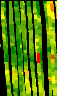
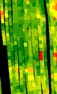
- Yield map interpretation is subjective. Differences in color schemes and selection of yield ranges can produce very different looking maps from the same data as shown in Figure 1 (Doerge, 1997). Likewise, yield map interpretations will vary with the experience level or bias of the practitioner.
|
|
|
|
Figure 1. Yield maps of the same field using two different theming methods. The map on the left uses yield ranges based on the standard deviation of the data set while the map on the right uses equal-interval theming. |
|
- The value of yield monitor data and maps extends beyond the year in which they were collected. Growers not only accumulate yield data and maps, but use this information to continually upgrade their agronomic, crop diagnostic and spatial data management skills.
- It is difficult to attribute improved farm outcomes to the practice of yield monitoring alone. Many other farm management competencies are needed to profit from the new kind of information provided by a yield map. For example, through yield monitoring a grower recognizes the adverse effect of weed competition on crop yield and successfully implements a more effective weed control program. Clearly the higher yields achieved were the result of yield monitoring as well as the effectiveness of the herbicide used and the grower’s skill in identifying, re-locating and treating the weed problem. This example demonstrates why it is nearly impossible to assess the economics of yield monitoring using traditional, controlled field experiments.
- Yield monitoring and mapping offer a wide variety of on- and off-farm profit opportunities that will vary from farm-to-farm and grower-to-grower. These include:
- real-time benefits during harvest
- much cheaper access to information from on-farm experimentation
- better variable-rate management
- quantitative evaluation of whole-field improvements such as tiling, windbreaks and irrigation, and
- enhancement of spatial and historical data bases and related management skills.
There is also an ever-increasing list of off-farm benefits such as more equitable landlord negotiations, identity preservation documentation for specialty end-use crops, "traceback" records for food safety, and documentation of environmental compliance.
The uncertainties in measuring the profitability of yield monitor use have resulted in the virtual absence of economic studies on this subject from university or industry sources. Nevertheless, yield monitors are being rapidly adopted by growers in the Corn Belt of North America and beyond. One Illinois survey projected that 42% of the growers polled in that survey plan to be yield monitoring by the year 2001 (Khanna, 1998). Growers apparently realize that yield monitoring has the potential to help them achieve improved farm profitability by saving inputs and increasing yields, but also by making them smarter managers.
Profit Opportunities Using a Yield Monitor
Currently, yield monitors measure or estimate two key harvest parameters on-the-go, grain moisture content and grain yield per acre. These measurements can be used to view crop yield variability trends on-the-go. After harvest, these data can be used to create detailed Field and Load Summaries. Addition of a differentially-corrected Global Positioning System (DGPS) receiver will allow the yield monitor to also log combine position from latitude and longitude readings taken every second. Yield and moisture data, plus the DGPS data can then be used to create yield and moisture maps as well as many other types of specialized maps. These include yield difference maps from a split-planter comparison, normalized yield maps which show within-field yield trends across different years and crops, and profit-loss maps.
The yield monitoring system can also be moved to other farm vehicles and be used to map planting, spraying, and cultivating activities, or virtually any other field operation. However, these various maps will be of limited value unless they are used appropriately and help the farm operator make beneficial management changes. Table 1 on page 4 summarizes some of the many ways that growers can use yield monitoring systems to increase their efficiency and overall profitability.
So… Should You Purchase a Yield Monitor?
Most growers with at least a minimum number of acres and years before retirement can profit from using a yield monitor, with or without DGPS capability. There may be no easier way to keep detailed field-by-field yield records than with a yield monitor. In addition, there are a number of in-field, real-time benefits as listed in Table 1 below that do not require a DGPS receiver. When deciding whether to add DGPS capability and start making yield maps, several additional questions should be considered:
- Are you willing to tackle the "yield monitoring learning curve", especially if you intend to do your own mapping and analysis?
- Do you have a strategy to manage the large quantity of spatial data that are generated by a yield monitor, either on your own computer or with the assistance of a qualified professional. (There are about 500,000 data records per 1500-acre farm per year).
- Are you willing to develop a complementary historical spatial data base over several years, to aid in the interpretation of yield maps? This includes one or more of the following: soil survey maps, soil electrical conductivity maps, bare soil and crop canopy aerial images, crop scouting reports and lab test results from geo-referenced soil samples.
Profiting from Yield Monitors in the Future
The opportunities to profit from yield monitor use will continue to increase in the future. This will occur as new and better sensors are developed and yield monitors become more integrated with other precision farming information systems. In the near future, better on-combine tools will be available to measure crop quality traits such as kernel quality and oil, protein and starch content. Eventually combines will be able to segregate grain based on these quality criteria and allow the grower to capture this value through identity preserved marketing. Software tools are even now being developed to enable much more powerful statistical and graphical analysis of multiple layers of spatial data. In addition, yield monitors will be linked to other information management systems that will assist with employee management and optimizing field operation logistics. Yield monitor data will eventually be useful as an input into new comprehensive crop simulation models that will help growers better manage production risk. Then as now, yield monitoring will make good growers better by giving them new information management tools to optimize inputs and outputs and better manage their farm operations.
References
Doerge, T. 1997. Yield map interpretation. Crop Insights Vol. 7, No. 25. Pioneer Hi-Bred International, Inc., Johnston, Iowa.
Doerge, T. 1998. Defining management zones for precision farming. Crop Insights Vol. 8, No. 21. Pioneer Hi-Bred International, Inc., Johnston, Iowa.
Khanna, M. 1998. Adoption of site-specific crop management: Current status and likely trends. Dept. of Agricultural and Consumer Economics, University of Illinois. Urbana, IL.
Marks, D. 1998. Iowa farmers slow to adopt precision farming. Iowa State University Extension Agricultural and Home Economics Experiment Station. Ames, IA.
Olson, K. 1998. Precision agriculture: Current economic and environmental issues. Dept. of Applied Economics, University of Minnesota. Posted on: @gInnovator, Agriculture Online. ( www.agriculture.com )
Swinton, S.M. and J. Lowenberg-DeBoer. 1998. Evaluating the profitability of site-specific farming. J. Prod. Agric. 11:439-446.
Wiebold, B., K. Sudduth, G. Davis, K. Shannon and N. Kitchen. Determining
barriers to adoption and research needs of precision agriculture. Report to the
North Central Soybean Res. Program. Missouri Precision Agriculture Center,
University of Missouri and USDA/ARS.
______________________________
Table 1. On- and off-farm profit opportunities that are available to growers using yield monitoring systems*.
|
Type of Profit Opportunity |
Examples |
|
In-Field, Real-Time Benefits During Harvest |
|
|
|
|
On-Farm Benefits |
|
|
|
|
Off-Farm Benefits |
|
|
|
*This list is not exhaustive and every grower may not realize all of these benefits due to site-specific differences in farm characteristics, local marketing opportunities and managerial expertise.
______________________________
Part 2. Investigating Interpolation Results
Comparing Interpolated and Extrapolated Data (return to top of Appendix A)
Table A.1 extends the residual analysis discussion in topic 2, "How Good Is My Map." It compares the results for interpolated data ("Interp")¾ data from estimated locations within the geographic bounds of the set of samples used in generating the map surfaces¾ and extrapolated data ("Extrap")¾ data from estimated locations outside the bounds.
Table A.1. Residual
analysis.
|
|
* Indicates
extrapolated estimates. Note that the sample size in the two populations is too
small to be confident about any analysis comparing them (number of
interpolations = 9 and number of extrapolations = 7).
That aside, table A.1 shows that all four techniques
have nearly equal or better "performance" for the interpolated
estimates than for the extrapolated ones. The Kriging technique is the exception, showing slightly better
performance for the extrapolated test set (Normalized .11 versus .12), but the
slight difference might simply be an artifact of the small sample size.
The average and inverse
techniques show about an 11 percent improvement for the interpolated estimates
versus the "Interp/Extrap" grouped results (.80 - .71 / .80 * 100 =
11.25%; .18 - .16 / .18 * 100 = 11.0%). The mincurve technique
shows less improvement (10.5%). The Kriging technique shows no
improvement for the interpolated set, but an 8 percent improvement for the
extrapolated set. Since this technique uses trends in the data, the results
seem to confirm that the trend extends beyond the geographic region of the
interpolation data set.
The tendency to underestimate was relatively
balanced for the average and Kriging techniques, with their "Sum of
Residuals" bias fairly equally split (-38 and -39 of -77; 13 and -15 of
-28). However, the inverse and mincurve techniques' biases were
relatively unbalanced (-9 and -20 of -29; -17 and -69 of -86) with an increased
tendency to underestimate the extrapolated values.
I wonder if there is a "significant difference" between the residuals for the interpolation and extrapolation estimates for each of the techniques? That's a fair question that requires a bit of calculation. The formulae for a t-test to see if the means of the two populations are different are shown in equations A.1 and A.2.
|
(Interp_Avg - Extrap_Avg) where, the Pooled Variance is
SUMSQ_Interp + SUMSQ_Extrap and variable processes are
|
The calculated t-test value is compared to values in a distribution of t table for the degrees of freedom (9-1 + 7-1 = 14, in this case) at various levels of significance. Let's see if there is a significant difference for the mincurve "Interp/Extrap" populations as shown in the following evaluation:
|
In this case, tabular t with 14
degrees of freedom at the 0.05 level is 2.145. Since our sample value
(1.10) is less than this, the difference is not significant at the 0.05
level. Anyone out there willing to test the average, inverse and Kriging
techniques to see if the "Interp/Extrap" estimates are
"significantly" different? (Show your work.)
Although the t-test is a good procedure to
test for significant differences in results, three requirements must be met for
it to be valid:
- random sample of residuals,
- residual values must be normally distributed and
- each group must have similar variances.
Number 1 was met since the residuals were
randomly sampled. Number 2 is a problem since the number of samples in
each group are small (9 and 7). Number 3 can be checked by
Bartlett's Test for homogeneity; and if group variances are deemed unequal, a
slightly different t-test is used.
The upshot of all this is that there
"appears" to be a difference between the levels of performance
(residuals) between the interpolated and extrapolated estimates, but we can't
say that there is a "statistically significant" difference between
the two for the mincurve map surface. Personally, I would attempt to
limit the proportion of extrapolated estimates in generating a map from point
data, particularly if I were using the inverse or mincurve techniques.
This means that the sampling design should "push" samples toward the
edge of the field and not start well within the field "just for symmetry."
Normalized Map Comparisons (return to top of
Appendix A)
|
|
|
Fig. A.2. Comparison of residual maps (2-D) using absolute
and normalized |
The maps discussed above were generated from the boo-boos (more formally termed residuals) uncovered by comparing interpolated estimates with a test set of known measurements. Numerical summaries of the residuals provided insight into the overall interpolation performance, whereas the map of residuals showed where the guesses were likely high and where they were likely low. The map on the left side of figure A.2 is the "plain vanilla" version. The one on the right is the normalized version. See any differences or similarities?
At first glance, the sets of lines seem to form radically different patterns—an extended thumb in the map on the left and a series of lilly-pads running diagonally toward the northeast in the map on the right. A closer look reveals that the patterns of the darker tones are identical. So what gives?
Defining the Norm (return to top of
Appendix A)
First of all, let's consider how the
residuals were normalized. The arithmetic mean of the test set (28) was
used as the common reference. For example, test location #17
estimated 2 while its actual value was 0, resulting in an overestimate of 2 by
subtraction (2 - 0 = 2). This simple residual is translated into a
normalized value of 7.1 by computing (0 - 2) / 28) * 100 = 7.1, a signed (+ or
-) percentage of the "typical" test value. Similar calculations
for the remaining residuals brings the entire test set in line with its
"typical value," then a residual map is generated (see eq. A.3).
|
Estimated
- Actual where Estimated
= estimated value from interpolation |
Now let's turn our attention back to the
maps. As the techy types among you guessed, the spatial pattern of
interpolation error is not effected by normalization (nor is its numerical
distribution)—all normalizing did was "linearly" re-scale the map
surface. The differences you detect in the line patterns are simply
artifacts of different horizontal "slices" through the two related
map surfaces. Whereas a 5-percent contour interval is used in the
normalized version, a contour interval of 1 is used in the absolute
version. The common "zero contour" (break between the two
tones) in both maps have an identical pattern, which would be the case for any
common slice (relative contour step).
Comparing the Comparable (return to top of
Appendix A)
If normalizing doesn't change a map surface,
why would anyone go to all the extra effort? Because normalizing provides
the consistent referencing and scaling needed for comparison among different
data sets. You can't just take a couple of maps, plop them on a light
table, and start making comparative comments. Everyone knows you have to
adjust the map scales so they will precisely overlay (spatial
registration). In an analogous manner, you have to adjust their
"thematic" scales as well. That's what normalization does.
Now visually compare magnitude and pattern of error between the Kriging and the average surfaces in figure A.3. A horizontal plane aligning at zero on the z-axis would indicate a "perfect" residual surface (all estimates were exactly the same as their corresponding test set measurements). The Kriging plot on the left is relatively close to this ideal, which confirms that the technique is pretty good at spatially predicting the sampled variable. The surface on the right, identifying the "whole field" average technique shows a much larger magnitude of error (surface deflection from z = 0). Now note the patterns formed by the light and dark blobs on both map surfaces. The Kriging overestimates (dark areas) are less pervasive and scattered along the edges of the field. The average overestimates occur as a single large blob in the southwestern half of the field.
|
|
|
Fig. A.3. Comparison of residual maps (3-D) using absolute and
normalized Kriging and |
What do you think you would get if you were
to calculate the volumes contained within the light and dark regions?
Would their volumetric difference have anything to do with their "Average
Unsigned Residual" values in the residual table, table A.1? What
relationship does the "Normalized Residual Index" have with the
residual surfaces? Bah! This map-ematical side of GIS really
muddles its comfortable cartographic side—bring on the colorful maps at
megahertz speed and damn the details.
Visually Comparing
Normalized Residual Maps (return to top of
Appendix A)
Figure A.4 compares the magnitude and pattern of the normalized residual maps of the averaging, inverse, Kriging and minimum curvature interpolation techniques. Table A.2 updates table A.1 with the normalized residual values (see eq. A.3) identified under the column heading "Pct."
|
|
|
|
|
Fig. A.4. Comparison of residual map surfaces (3-D) using residual
values derived by Kriging, inverse, |
The 3-D plots of the residual surfaces in figure A.3 dramatically show the relative magnitude of errors associated with four surface modeling techniques. A horizontal plane positioned at z = 0 would characterize a perfect data model (all estimates equal to their corresponding test measurements; 0 total error). The magnitude of the deflections from this ideal indicate the amount of error.
A horizontal plane "fitted" to a
residual surface (half above and half below) should track the arithmetic
average of the residuals, and thereby approximate the average of the
interpolated estimates. For example, you would expect the fitted plane on
the Kriging surface to "balance" at -7.1 percent ("K_Est
Average" of 26 is 2 residual units below the test average of 28 (-2 / 28)
* 100 = -7.1). The fitted plane for the other surfaces would approach:
"Average" = -17.9%, "Inverse" = -7.1%, and
"MinCurve" = 21.4%.
Note that the "Estimate Average"
depicted in table A.2 provides very little insight into magnitude and pattern
of errors, simply how well the over/under estimates compensate. Although the
average surface contains a lot more error, it is better balanced than the
mincurve surface (17.9 percent versus 21.4 percent).
Table A.2. Normalized residual analysis.
|
|
* Indicates
extrapolated estimates
The total volume above the "zero
plane" identifies overestimates; the total volume below it identifies
underestimates. The net volume between the two approximates the
arithmetic "Sum of the Residuals." The sign of the net volume
indicates an over (+) or under (-) bias in the estimates, while the size of the
volume indicates the relative amount of bias. In the case of the mincurve
surface it has substantial error (overall volume), which is balanced well below
the test set average—large underestimating bias. Errors of this nature
are particularly troublesome. If you were a farmer applying fertilizer
according to the mincurve "prescription," you could be vastly under
applying throughout the field.
The total volume of the deflections of the
surface above and below the zero plane identify total (unsigned) error of the
estimated map. The "Average Unsigned Residual" is equivalent to
simply proportioning the total error volume by the number test samples (number
of sample = 16). An analogous spatial proportioning subdivides the field
into 16 equal-area parcels and characterizes the error in each. Instead
of assuming the "typical" error is the same throughout the field, the
spatially based partitioning provides a glimpse at its spatial distribution.
This "course" treatment of error might be useful if a farmer
has equipment that can't respond to all the detail in the estimated surface
itself—at least he would have 16 areas that could respond to "tweaking"
a fertilizer prescription based on probable error of the estimate within each
parcel. Since the residual surfaces were all normalized at the onset, the
"Normalized Residual Index" identified in table A.1 is redundant.
The positioning of the deflections from the
ideal characterize the pattern of error and is best viewed in 3-D (see fig.
A.4). Note the similarity in the patterns of the light (-) and dark (+)
tones between the inverse and average residual surfaces. Although the
magnitudes of error are radically different (contour spacing), the under/over
transition lines are almost identical splitting the field into two blobs ( SE
from the NE).
The Kriging and mincurve surfaces contain a
few scattered overestimate blobs that show minimal spatial coincidence.
These similarities and differences in pattern are likely the result of the
different interpolation algorithms. The average technique simply computes
the average of the set of interpolation samples, then spatially characterizes
it as a horizontal plane (a flat surface of 23 everywhere). The
inverse-distance algorithm uses a weighted moving average with closer samples
influencing individual estimates more than distant ones. Both algorithms
are based on overall averaging independent of directional and localized trends.
The Kriging and mincurve techniques incorporate both extended factors, but in
different ways forming more complex residual surfaces. Note that the
"Kriging/Inverse" (best) and "MinCurve/Average" (worst)
pairing¾considering similarities in error magnitude¾switch to an "Inverse/Average" (clumped) and
"Kriging/MinCurve" (dispersed) pairing, when considering error
patterns.
Also, keep in mind that generalized
conclusions about interpolation techniques are invariably wrong because the
nature of interpolation errors are dependent on a complex interaction of
sampling design, sample values themselves, interpolation technique and the
algorithm parameters. That's why you should always construct a residual
analysis table and a set of normalized residual maps before you select and
store a map generated from point samples in your GIS.
The normalized residuals are identified under the column heading "Pct." They were normalized to the arithmetic average of the test set of data (28) in equation A.3 of percent difference. The sets of normalized residuals were interpolated using the inverse distance technique to generate the residual maps shown in figure A.4. It is recommended that the residuals be normalized before tabular or map comparison among different interpolation or sampling techniques applied to common interpolation and test sets.
More on Zones and Surfaces (return to top of
Appendix A)
The previous section identified the
similarities and differences in the characterization of field data by
"Management Zones" and "Map Surfaces." Recall that
both approaches carve a field into smaller pieces to better represent the
unique conditions and patterns occurring in the field. Zones partition it into
relatively large, irregular areas that are assumed to be homogenous.
Field samples (e.g., soil samples) are extracted and the average for each
factor is assigned to the entire zone—discrete polygons. Surfaces, on the
other hand, interpolate field samples for an estimate of each factor at each
grid cell in a uniform analysis grid—continuous gradient.
|
|
|
Fig. A.5. Comparison of management zones and map surface
representations |
The left side of figure A.5 shows an overlay
of surface grids and management zones for the field. The three management
zones are divided into eight individual clumps—four for zone 1 and two for
zones 2 and 3.
The map surface for the same area is composed
of 1,380 grid cells configured as an analysis grid of 46 rows by 30
columns. Each zone contains numerous grid cells—from Clump #1 with only
11 cells to Clump #5 with nearly 800. While a single value is assigned to
all of the clumps comprising a zone, each grid cell is assigned a value that
best represents the field data collected in its vicinity. The subtle (and
not so subtle) differences within zones and their individual clumps are
contained within the grid values defining the continuous map surface.
The right side of the figure summarizes these
differences. The maps at the top show the alignment of the
"Management Zones" with the "Map Surface." Note the
big bump on the surface occurring in Clump #2 (northeast corner) of Zone 1
(darkest tone). Note the big hole next to it at the top of Clump #7 of
Zone 3 and the "wavy" pattern throughout the rest of the clump.
Although these and less obvious surface variations are lost in the zone
averages, the zones and surface patterns have some things in common—Zone 1
tends to coincide with the higher portions of the surface, Zone 2 a bit lower
and Zone 3 the lowest.
Now consider the summary table. The average
for Zone 1 (all four clumps) is 55, but there’s a fair amount of variation in
the grid values defining the same area—ranging from 29 to 140. Its coefficient of variation (Coffvar) of 34% warns us that the zone average isn’t
very typical. The bumpiness of the dark toned areas on the surface
visually confirms the same thing. Note that of all the clumps, Clump #2
has the largest internal variation (values from 43 to 140, Coffvar of 31% and
the largest bump). Clump #1 has the least internal variation (values from
40 to 43, Coffvar of only 2% and nearly flat). A similar review of the
tabular statistics and surface plot for the other whole zones and individual
clumps highlight the differences between the two approaches.
Site-specific management assumes reliable
characterization of the spatial variation in a field. Whereas
"Management Zones" may account for more variation than "Whole
Field" averages, the approach fails to map the variation within the zones.
The next section investigates the significance of this limitation.
Last Word on Zones and Surfaces (return to top of
Appendix A)
While much of the information in a GIS is
discrete, such as the infrastructure of roads, buildings, and power lines, the
focus of many applications, including precision farming, extend to decision
factors that widely vary throughout geographic space. As a result,
surface modeling plays a dominant role in site-specific management of such
geographically diffuse conditions.
Map surfaces (formally termed spatial gradients) are characterized
by grid-based data structures. In forming a surface, the traditional
geographic representation based on irregular polygons is replaced by a highly
resolved matrix of uniform grid cells superimposed over an area (see the top
portion of fig. A.6).
|
|
|
Fig. A.6. Comparison of zone (polygon) and surface (grid)
representations for a |
The data range representation for the two
approaches are radically different. Consider the alternatives for
characterizing phosphorous levels throughout a field. Zone management, uses air photos and a farmer’s knowledge to
subdivide the field into similar areas (gray levels on the left side of fig.
A.6). Soil samples are randomly collected in the areas and the average
phosphorous level is assigned to each zone. A complete set of soil
averages is used to develop a fertilization program for each zone in the field.
Site-specific management, on the other hand, systematically samples the field
and interpolates these data for a continuous map surface (right side of fig.
A.6). First, note the similarities between the two representations—the
generalized levels (data range) for the zones correspond fairly well with the
map surface levels with the darkest zone generally aligning with higher surface
values, while the lightest zone generally corresponds to lower levels.
Now consider the differences between the two
representations. Note that the zone approach assumes a constant level
(horizontal plane) of phosphorous throughout each zone—Zone #1 (darkgray) = 55,
Zone #2 = 46 and Zone #3 (lightgray) = 42—while the map surface shows a
gradient of change across the entire field that varies from 22 to 140.
Two important pieces of information are lost in the zone approach—the extreme
high/low values and the geographic distribution of the variation. This
"missing" information severely limits the potential for further
analysis of the zone data.
The loss in spatial specificity for a map
variable by generalizing it into zones can be significant. However, the
real kicker comes when you attempt to analyze the coincidence among maps.
Figure A.7 shows three geo-referenced surfaces for the field as phosphorous
(P), potassium (K) and acidity (PH). The pins depict four of the 1380
possible combinations of data for the field. By contrast, the zonal
representation has only three possible combinations since it has just three
distinct zones with averages attached.
The assumption of the zone approach is that
the spatial coincidence (alignment) of the averages is consistent throughout
the field. If there is a lot of spatial dependency among the variables
and the zones happen to align with actual patterns in the data, this assumption
holds. However, in reality, good alignment for all of the variables is
not always the case.
|
|
|
Fig. A.7. Geo-referenced map surfaces |
|
Table A.3. Comparison of zone and surface data for selected locations. |
|
|
Consider the "shishkebab" of data
values for the four pins shown in table A.3. The first two pins are in
Zone #1, so the assumption is that the levels of phosphorous = 55, potassium =
457 and acidity = 6.4 are the same for both pin locations (as they are for all
locations within Zone #1). But the surface data for Pin #1 indicates a
sizable difference from the averages—150% ( ( (140-55) / 55) * 100) for phosphorous,
28% for potassium and 8% for acidity. The differences are less for Pin #2
with 20%, 2% and –2%, respectively. Pins #3 and #4 are in different
zones, but similar deviations from the averages are noted, with the greatest
differences in phosphorous levels and the least in acidic levels. It
follows that different fields likely have different "alignments"
between the zones and surfaces—some good and some bad.
The pragmatic arguments of minimal sampling
costs and conceptual simplicity, however, favor zone management, provided the
objective is to forego site-specific management and "carve" a field
into presumed homogenous, bite-sized pieces. One can argue that even an
arbitrary sub-division of a field often can lower the variance in each
section—at least if the driving variables aren't uniformly or randomly
distributed across the field (i.e., no spatial autocorrelation).
Most field boundaries are expressions of
ownership and historical farm practices. The appeal of sub-dividing
these arguably arbitrary parcels into more management-based units is
compelling, particularly if the parsing results in significantly lower sampling
costs.
However, site-specific management is more
than simply breaking a field into smaller, more intuitive zones. It is
deriving relationships among agronomic variables and farm inputs/actions that
are unique to a field. An important limitation of zone management is that
it assumes ideal stratification of a field at the onset of data collection,
analysis and determining appropriate action—in scientific-speak, spatially
biasing the process.
Since the discrete zones are assumed
homogenous at the onset, tests of that assumption and any further spatial
analysis is usurped. What if the intuitive zones don't align with the
actual soil fertility levels currently in the soil? Does it make sense to
manage fertility levels within intuitive zones that are primarily determined by
water management, variety response, localized disease/insect pockets or other
processes? Would two different consultant/farmer teams draw the same
lines for a given field? Or for that matter, would an aerial photo taken
a couple of days after a storm show the same bare-soil patterns as one taken
several weeks after the last rainfall? Do zones derived by electrical
conductivity mapping align with aerial photo-based ones? What might cause
the differences in zone maps generated by the two approaches and which one more
closely aligns with the actual variation in soil nutrient levels? What is
the appropriate minimum mapping unit (smallest "circled" area) for a
zone? What is the appropriate number of zones (low, medium, high)?
Is the low productivity in a slight depression due to variety intolerance,
disease susceptibility or fertility? What about the yield inconsistencies
on the hummocks?
Zone management is unable to address any of
these questions as it fails to collect the necessary spatial data.
Although zone sampling is inexpensive, a simple average assigned to each zone
fails to leave a foothold for assessing how well the technique is tracking the
actual patterns in a field. Nor does it provide any insights into the
unique and spatially complex character of most fields.
In addition, management actions (e.g.,
fertilization program) are developed using generalized relationships (largely
based on research developed years ago at an experiment station miles away) and
applied uniformly over each zone regardless of the amount or pattern of its
variance in soil samples. What if crop variety responds differently on the
subtle (and not so subtle) differences between the research field and the
actual field? What if there are fairly significant differences in
micro-topography between the fields? What about the pattern and extent of
soil texture differences? Are seeding rates and cultivation practices the
same?
Zone management follows in the tradition of
the whole-field approach—sort of a "whole-zone" approach. It’s
likely a step in the right direction, but how far? And do the assumptions
apply in all cases? How much of a field’s reality (spatial variability)
is lost in averaging? There is likely a myriad of interrelated
"zones" within a field (water, microclimate, terrain, subsurface
flows, soil texture, microorganisms, fertility, etc.) depending on what variable
is under consideration. The assumption that there is a single distinct
and easily drawn set of polygons that explain crop response doesn't always
square with GIS or agronomic logic.
Current zoning practices contain both art and
science. Like herbal cures, zone management holds significant promise but needs
to be validated and perfected. Simply justifying the approach as a
remedy to the "high cost of entry" to precision farming without
establishing its scientific underpinnings could make it a low-cost, snake-oil
elixir in high-tech trappings. The advice of the Great and All-powerful
Oz might hold. "Pay no attention to the man behind the curtain"
at least until minimal data analysis proves the assumptions hold true on your
farm.
Excel Worksheets Investigating Zones and Surfaces (return to top of
Appendix A)
Excel worksheets supporting the discussions
of spatial dependency are available online. You need access to the Excel
program or similar spreadsheet system that can read Excel97 files.
Note: Download files are self-extracting
PKZip files. To unarchive, save the file, then open it (double-click
from Explorer) and the original file will be extracted to the folder containing
the zip file.
|
Topic 2: "Zones and Surfaces" |
|
|
|
|
______________________________
Part 3. More on Spatial Dependency
Spatial Dependency and Distance (return to top of
Appendix A)
As discussed in topic 3, "Assessing Spatial
Dependency," nearest-neighbor spatial dependency tests the assertion
that "nearby things are more related than distant things."
The procedure is simple— calculate the unsigned difference between each sample
value and its closest neighbor (|Value - NN_Value|), then compare them
to the differences based on the typical condition (|Value - Average|).
If the nearest-neighbor and average differences are about the same, little
spatial dependency exists. If the nearby differences are substantially
smaller than the typical differences, then strong positive spatial dependency
is indicated and it is safe to assume that nearby things are more related.
But just how are they related? And just
how far is "nearby?" To answer these questions the procedure
needs to be expanded to include the differences at the various distances
separating the samples. As with the previous discussions, Excel can be
used to investigate these relationships.* The plot on the left side of
figure A.8, identifies the positioning and sample values for the "Tilted
Plane" data set described in topic 3, "Assessing Spatial
Dependency."
|
|
|
Fig. A.8. Spatial dependency as a function of distance for sample point #1. |
The arrows emanating from sample #1 shows its
15 paired values. The table on the right summarizes the unsigned
differences (|Diff |) and distances (Distance)
for each pair. Note that the "nearby" differences (e.g., #3 =
4.0, #4 = 5.0 and #5 = 4.0) tend to be much smaller than the
"distant" differences (e.g., #10 = 17.0, #14 = 22.0, and #16 =
18.0). The graph in the upper right portion of the figure plots the
relationship of sample differences versus increasing distances. The
dotted line shows a trend of increasing differences (i.e., dissimilarity)
with increasing distances.
Now imagine calculating the differences for
all the sample pairs in the data set—the 16 sample points combine for 125
sample pairs. Admittedly, these calculations bring humans to their knees,
but it's just a microsecond or so for a computer. The result is a table
containing the |Diff | and Distance values for all of the sample
pairs.
The extended table embodies a lot of
information for assessing spatial dependency. The first step is to
divide the samples into two groups, close and distant pairs. By
successively increasing the breakpoint, the sample values falling in the
"nearby" and "distant" neighborhoods around each sample
location change. This approach allows us to directly assess the essence
of spatial dependency—whether nearby things are more related than distant
things—through a distance-based spatial dependency measure (SD_D)
calculated in equation A.4.
|
|Avg_Distant| - |Avg_Nearby| where
"| ... |" indicates absolute value (i.e., unsigned value treated as
positive in the equation) |
The effect of this processing is like passing
a donut over the data. When centered on a sample location, the
"hole" identifies nearby samples, while the "dough"
determines distant ones. The "hole" gets progressively larger
with increasing breakpoint distances. If, at a particular step, the
nearby samples are more related (smaller |Avg_Nearby| differences) than
the distant set of samples (larger |Avg_Distant| differences), positive
spatial dependency is indicated.
|
|
|
Fig. A.9. Comparing spatial dependency by directly assessing differences of a sample's value to those within nearby and distant sets. |
Now let’s put the SD_D measure to use.
Figure A.9 plots the measure at several breakpoints for the same tilted plane
(TP with constantly increasing values) and jumbled placement (JP with a jumbled
arrangement of the same values) data used last month. First, notice that
the measures for TP are positive for all breakpoint distances (nearby things
are always more related), whereas they bounce around zero for the JP
pattern. Next, notice the magnitudes of the measures— fairly large for TP
(big differences between nearby and distant similarities), fairly small for
JP. Finally, notice the trend in the plots—downward for TP (declining
advantage for nearby neighbors), flat or unpredictable for JP.
So what does all this tell us? If the
sign, magnitude and trend of the SD_D measures are like TP’s, then positive
spatial dependency is indicated and the data conforms to the underlying
assumption of most spatial interpolation techniques. If the data is more
like JP, then "interpolator beware."
Note: The Excel worksheet supporting this
discussion is available online; see appendix A, part 2, Excel
Worksheets Investigating Spatial Dependency.
Mapping Spatial Dependency (return to top of
Appendix A)
The previous discussion identifies how to
test if nearby things are more related than distant things in sets of
discrete sample points, such as soil samples from a field. Now let’s turn
our attention to continuously mapped data, such as crop yield and remote
sensing data.
|
|
|
Fig. A.10. Spatial dependency in continuously mapped data
involves |
As depicted in figure A.10, an instantaneous
moment in the processing establishes a set of neighboring cells about a map
location. The map values for the center cell and its neighbors are
retrieved from storage and depending on the analysis technique, the values are
summarized. The window is shifted so it centers over the next cell and
the process is repeated until all map locations have been evaluated.
If two cells are close together and have
similar values they are considered spatially related; if their values are
different, they are considered unrelated, or even negatively related.
Geary’s C (eq. A.5) and Moran’s I (eq. A.6) are
the most frequently used measures for determining spatial autocorrelation in
mapped data. Although the equations are a bit intimidating,
|
[(n –1) SUM wij
(xi – xj)2] [n
SUM wij (xi – m) (xj – m)] where,
n = number of cells in the grid |
the underlying concept is fairly simple.
For example, the Geary’s C equation simply
compares the squared differences in values between the center cell and its
adjacent neighbors (numerator tracking xi – xj)
to the overall difference based on the mean of all the values (denominator
tracking xi – m). If the adjacent differences are
less, then things are positively related (similar, clustered). If they
are more, then things are negatively related (dissimilar, checkerboard).
And if the adjacent differences are about the same, then things are unrelated
(independent, random). The Moran’s I equation is a similar measure, but relates
the product of the adjacent differences to the overall difference.
Now let’s do some numbers. An adjacent
neighborhood consists of the four contiguous cells about a center cell, as
highlighted in the upper right inset of figure A.7. Given that the mean
for all of the values across the map is 170, the essence for this piece of
Geary’s puzzle is
C =
[(146-147)2 + (146-103) 2 + (146-149) 2 +
(146-180) 2] / [4 * (146-170) 2]
= [ 1 + 1849 + 9 + 1156 ] / [ 4 * 576 ] = 3015 /2304 = 1.309
Since the ratio is just a bit more than 1.0,
a slightly uncorrelated spatial dependency is indicated for this
location. As the window completes its pass over all of the other cells,
it keeps a running sum of the numerator and denominator terms at each location.
The final step applies some aggregation adjustments to calculate a single
measure encapsulating spatial autocorrelation over the whole map— a Geary’s C
of 0.060 and a Moran’s I of 0.943 for the map surface shown in the figure.
Both measures report strong positive autocorrelation for the mapped
data. The general interpretation of the C and I statistics can be
summarized in table A.5.
Table A.5.
Interpreting Geary's C and Moran's I calculated values.
|
0 < C < 1 |
Strong positive autocorrelation |
I > 0 |
|
C > 1 |
Strong Negative autocorrelation |
I < 0 |
|
C = 1 |
Random distribution of values |
I = 0 |
In the tradition of good science, let me
suggest a new, related measure—Berry’s ID. This intuitive
dependency (ID) measure simply assigns the calculated ratio from Geary’s
formula to each map location. The result is a map indicating the spatial
dependency for each location (pieces of the puzzle), instead of a single value
summarizing the entire map. In the "Adjacent Neighbors" table
in figure A.6, 1.309 is assigned to the center location in the figure.
However a value of 0.351 is assigned to the cell directly above it and 4.675 is
assigned to the cell directly below it—you do the math.
Although this new measure might be intuitive
there are other more statistically robust approaches. Consider the
"Doughnut Neighborhood" comparison in the figure. The roving
window is divided into two sets of data—the adjacent values (inside ring of nearby
things) and the doughnut values (outside ring of distant things).
One can directly assess whether nearby things are more related than distant
things by evaluating the differences in both rings. An even more
advance approach compares the F-values within each ring to test for significant
difference.
Although the math/stat is a bit confusing for
all but the techy-types, the concept is fairly simple and easy to
implement. But is it useful? You bet. A spatial dependency
map shows you where things (i.e., yield or soil nutrients) are strongly related
and where they’re not. If they are, then management actions can be
consistently applied. If they’re not, then more information is
needed. At least you know where things vary a lot and when they are
fairly unpredictable and you had better watch out.
Note: The Excel worksheet supporting this
discussion is available online; see appendix A, part 2, Excel
Worksheets Investigating Spatial Dependency.
Excel Worksheets
Investigating Spatial Dependency (return to top of
Appendix A)
Excel worksheets supporting the discussions
of spatial dependency are available online. You need access to the Excel
program or similar spreadsheet system that can read Excel97 files.
Note: Download files are self-extracting
PKZip files. To unarchive, save the file, then open it (double-click
from Explorer) and the original file will be extracted to the folder containing
the zip file.
|
Topic 3: "Assessing Spatial Dependency" |
|
|
|
|
|
Appendix A, Part 3: "Spatial Dependency and Distance" |
|
|
|
|
|
______________________________
Part 4. More on Correlation and
Comparing Map Surfaces
Excel Worksheet
Investigating Map Correlation and Prediction (return to top of
Appendix A)
An Excel worksheet supporting the discussions
on map correlation and predictive modeling are available online. You
need access to the Excel program or similar spreadsheet system that can read
Excel97 files.
Note: Download files are self-extracting
PKZip files. To unarchive, save the file, then open it (double-click
from Explorer) and the original file will be extracted to the folder containing
the zip file.
|
Topic 4: "Map Correlation and Prediction" |
|
|
|
|
Validity of Using Statistical Tests with mapped Data (return to top of
Appendix A)
By William Huber, PhD
Quantitative Decisions, Merion Station, PA
To be completed.
Excel Worksheet Investigating Map Surface Comparison (return to top of
Appendix A)
An Excel worksheet supporting the discussions
on comparing map surfaces are available online. You need access to the
Excel program or similar spreadsheet system that can read Excel97 files.
Note: Download files are self-extracting
PKZip files. To unarchive, save the file, then open it (double-click
from Explorer) and the original file will be extracted to the folder containing
the zip file.
|
Topic 4: "Comparing Map Surfaces" |
|
|
|
|