An
Analytical Framework for GIS Modeling
Joseph
K. Berry1 and Shitij Mehta2
1Keck Scholar in Geosciences, Department of
Geography, University of Denver, Denver, Colorado; jkberry@du.edu Website: www.innovativegis.com/basis/
2Former Graduate Teaching Assistant at the
University of Denver; currently Product Engineer, Geoprocessing
Team, Environmental Systems Research Institute (ESRI), Redlands, California
Abstract:
The U.S.
Department of Labor has identified Geotechnology as
one of three mega technologies for the 21st century noting that it
will forever change how we will conceptualize, utilize and visualize spatial
information. Of the spatial triad
comprising Geotechnology (GPS, GIS and RS), the spatial analysis and modeling
capabilities of Geographic Information Systems provides the greatest untapped
potential, but these analytical procedures are least understood. This paper develops a conceptual framework
for understanding and relating various grid-based map analysis and modeling
procedures, approaches and applications.
Discussion topics include; 1) the nature of discrete versus continuous
mapped data; 2) spatial analysis procedures for reclassifying and overlaying
map layers; 3) establishing distance/connectivity and depicting neighborhoods; 4) spatial statistics procedures for surface
modeling and spatial data mining; 5) procedures for communicating model
logic/commands; and, 6) the impact of spatial reasoning/dialog on the future of
Geotechnology.
Keywords:
Geographic Information Systems, GIS modeling, grid-based map analysis, spatial
analysis, spatial statistics, map algebra, map-ematics
This
paper presents a conceptual framework used in organizing material presented in
a graduate course on GIS Modeling presented at the University of Denver. For more information and materials see http://www.innovativegis.com/basis/Courses/GMcourse11/.
Posted
November, 2011
<Click here>
for a printer- friendly version of this paper (.pdf)
|
Table
of Contents |
||
|
Section |
Topic |
Page |
|
Introduction |
2 |
|
|
Nature of Discrete
versus Continuous Mapped Data |
4 |
|
|
Spatial Analysis
Procedures for Reclassifying Maps |
6 |
|
|
Spatial Analysis
Procedures for Overlaying Maps |
8 |
|
|
Spatial Analysis
Procedures for Establishing Proximity and Connectivity |
10 |
|
|
Spatial Analysis Procedures
for Depicting Neighborhoods |
13 |
|
|
Spatial Statistics
Procedures for Surface Modeling |
15 |
|
|
Spatial Statistics
Procedures for Spatial Data Mining |
17 |
|
|
Procedures for
Communicating Model Logic |
18 |
|
|
Impact of Spatial
Reasoning and Dialog on the Future of Geotechnology |
20 |
|
|
|
Further Reading and
References |
23 |
____________________________
Historically information relating to
the spatial characteristics of infrastructure, resources and activities has
been difficult to incorporate into planning and management. Manual techniques of map analysis are both
tedious and analytically limiting. The
rapidly growing field of Geotechnology
involving modern computer-based systems, on the other hand, holds promise in
providing capabilities clearly needed for determining effective management
actions.
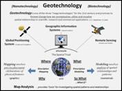
Geotechnology refers to
“any technological application that utilizes spatial location in visualizing, measuring,
storing, retrieving, mapping and analyzing features or phenomena that occurs
on, below or above the earth” (Berry, 2009).
It is recognized by the U.S. Department of Labor
as one of the “three mega-technologies for the 21st Century,” along
with Biotechnology and Nanotechnology (Gewin,
2004). As depicted in the left inset of
figure 1 there are three primary mapping disciplines that enable Geotechnology—
GPS (Global Positioning System)
primarily used for location and navigation, RS
(Remote Sensing) primarily used to measure and classify the earth’s cover,
and GIS (Geographic Information
Systems/Science/Solutions) primarily used for mapping and analysis of
spatial information.
The interpretation of the “S” in GIS
varies from “Systems” with an emphasis on data management and the computing
environment. A “Science” focus
emphasizes the development of geographic theory, structures and processing
capabilities. A “Solutions” perspective
emphasizes application of the technology within a wide variety of disciplines
and domain expertise.
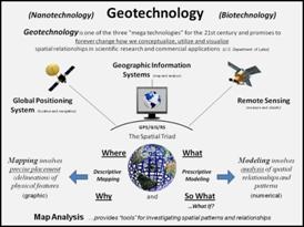
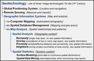
Figure 1. Overview organization of components, evolution and types of tools
defining Map Analysis.
Since the 1960s the
decision-making process has become increasingly quantitative, and mathematical
models have become commonplace. Prior to
the computerized map, most spatial analyses were severely limited by their
manual processing procedures. Geographic
information systems technology provides the means for both efficient handling
of voluminous data and effective spatial analysis capabilities. From this perspective, GIS is rooted in the
digital nature of the computerized map.
While today’s
emphasis in Geotechnology is on sophisticated multimedia mapping (e.g., Google Earth, internet mapping, web-based
services, virtual reality, etc.), the early 1970s saw computer mapping as a high-tech
means to automate the map drafting process.
The points, lines and areas defining geographic features on a map are
represented as an organized set of X,Y
coordinates. These data drive pen
plotters that can rapidly redraw the connections at a variety of colors,
scales, and projections. The map image,
itself, is the focus of this automated cartography.
During the early
1980s, Spatial database management systems
(SDBMS) were developed that linked computer mapping capabilities with
traditional database management capabilities.
In these systems, identification numbers are assigned to each geographic
feature, such as a timber harvest unit or sales territory. For example, a user is able to point to any
location on a map and instantly retrieve information about that location. Alternatively, a user can specify a set of
conditions, such as a specific vegetation and soil combination, and all
locations meeting the criteria of the geographic search are displayed as a map.
As Geotechnology
continued its evolution, the 1990s emphasis turned from descriptive “geo-query”
searches of existing databases to investigative Map Analysis. Today, most GIS
packages include processing capabilities that relate to the capture, encoding,
storage, analysis and visualization of spatial data. This paper describes a conceptual framework
and a series of techniques that relate specifically to the analysis of mapped
data by identifying fundamental map analysis operations common to a broad range
of applications. As depicted in the
lower portion of the right inset in figure 1, the classes of map analysis
operations form two basic groups involving Spatial
Analysis and Spatial Statistics.
Spatial Analysis extends the basic set of discrete map features of points, lines and
polygons to surfaces that represent continuous geographic space as a set of
contiguous grid cells. The consistency
of this grid-based structuring provides a wealth of new analytical tools for
characterizing “contextual spatial relationships,” such as effective distance,
optimal paths, visual connectivity and micro-terrain analysis. Specific classes of spatial analysis
operations that will be discussed include Reclassify,
Overlay, Proximity and Neighbors.
In addition, it
provides a mathematical/statistical framework by numerically representing
geographic space. Whereas traditional
statistics is inherently non-spatial as it seeks to represent a data set by its
typical response regardless of spatial patterns, Spatial Statistics
extends this perspective on two fronts.
First, it seeks to map the variation in a data set to show where unusual
responses occur, instead of focusing on a single typical response. Secondly, it can uncover “numerical spatial
relationships” within and among mapped data layers, such as generating a
prediction map identifying where likely customers are within a city based on
existing sales and demographic information.
Specific classes of spatial statistics operations that will be discussed
include Surface Modeling and Spatial Data Mining.
By organizing primitive analytical
operations in a logical manner, a generalized GIS modeling approach can be
developed. This fundamental approach can
be conceptualized as a “map algebra” or “map-ematics”
in which entire maps are treated as variables (Tomlin and Berry, 1979; Berry,
1985; Tomlin, 1990). In this context,
primitive map analysis operations can be seen as analogous to traditional
mathematical operations. The sequencing
of map operations is similar to the algebraic solution of equations to find
unknowns. In this case however, the
unknowns represent entire maps. This
approach has proven to be particularly effective in presenting spatial analysis
techniques to individuals with limited experience in geographic information
processing.
2.0 Nature of Discrete versus Continuous Mapped
Data
For
thousands of years, points, lines and polygons have been used to depict map
features. With the stroke of a pen a
cartographer could outline a continent, delineate a highway or identify a specific
building’s location. With the advent of
the computer and the digital map, manual drafting of spatial data has been
replaced by the cold steel of the plotter.
In
digital form, mapped data have been linked to attribute tables that describe
characteristics and conditions of the map features. Desktop mapping exploits this linkage to
provide tremendously useful database management procedures, such as address
matching, geo-query and network routing.
Vector-based data forms the foundation of these techniques and
directly builds on our historical perspective of maps and map analysis.
Grid-based data, on
the other hand, is a less familiar way to describe geographic space and its
relationships. At the heart of this
procedure is a new map feature that extends traditional irregular discrete Points, Lines and Polygons
(termed “spatial objects”) to uniform continuous map Surfaces.
The
top portion of figure 2 shows an elevation surface displayed as a traditional
contour map, a superimposed analysis frame and a 2-D grid map. The highlighted location depicts the
elevation value (500 feet) stored at one of the grid locations. The pop-up table at the lower-right shows the
values stored on other map layers at the current location in the Analysis Frame. As the cursor is moved, the “drill-down” of
values for different grid locations in the Map
Stack are instantly updated.
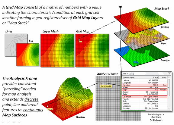
Figure 2.
Grid-based map layers form a geo-registered stack of maps that are
pre-conditioned for map analysis.
Extending
the grid cells to the relative height implied by the map values at each
location forms the 3-dimensional plot in the lower-left portion of the
figure. The result is a “grid” plot that
depicts the peaks and valleys of the spatial distribution of the mapped data
forming the surface. The color zones
identify contour intervals that are draped on the surface. In addition to providing a format for storing
and displaying map surfaces, the analysis frame establishes the consistent
structuring demanded for advanced grid-based map analysis operations. It is the consistent and continuous nature of
the grid data structure that provides the geographic framework supporting the
toolbox of grid-based analytic operations used in GIS modeling.
In
terms of data structure, each map layer in the map stack is comprised of a
title, certain descriptive parameters and a set of categories, technically
referred to as Regions. Formally stated, a region is simply one of
the thematic designations on a map used to characterize geographic
locations. A map of water bodies
entitled “Water,” for example might include regions associated with dry land,
lakes or ponds, streams and wetlands.
Each region is represented by a name (i.e., a text label) and a
numerical value. The structure described so far, however, does not account for
geographic positioning and distribution.
The handling of positional information is not only what most
distinguishes geographic information processing from other types of computer
processing; it is what most distinguishes one GIS system from another.
As
mentioned earlier, there are two basic approaches in representing geographic
positioning information: Vector, based on sets of discrete line segments, and
Raster, based on continuous sets of grid cells.
The vector approach stores information about the boundaries between
regions, whereas raster stores information on interiors of regions. While this difference is significant in terms
of implementation strategies and may vary considerably in terms of geographic
precision, they need not affect the definition of a set of fundamental
analytical techniques. In light of this
conceptual simplicity, the grid-based data structure is best suited to the
description of primitive map processing techniques and is used in this
paper.
The
grid structure is based on the condition that all spatial locations are defined
with respect to a regular rectangular geographic grid of numbered rows and
columns. As such, the smallest
addressable unit of space corresponds to a square parcel of land, or what is
formally termed a Grid Cell, or more
generally referred to as a “point” or a “location.” Spatial patterns are represented by assigning
all of the grid cells within a particular region a unique Thematic Value. In this way,
each point also can be addressed as part of a Neighborhood of surrounding values.
If
primitive operations are to be flexibly combined, a processing structure must
be used that accepts input and generates output in the same format. Using the data structure outlined above, this
may be accomplished by requiring that each analytic operation Involve—
- retrieval of
one or more map layers from the map stack,
- manipulation of
that mapped data,
- creation of a
new map layer whose categories are represented by new thematic values
derived as a result of that manipulation, and
- storage of that
new map layer back into the map stack for subsequent processing.
The cyclical nature of the
retrieval-manipulation-creation-storage processing structure is analogous to
the evaluation of “nested parentheticals” in traditional algebra. The logical sequencing of primitive map
analysis operations on a set of map layers forms a spatial model of specified
application. As with traditional
algebra, fundamental techniques involving several primitive operations can be
identified (e.g., a “travel-time map”) that are applicable to numerous
situations.
The use of these primitive map
analysis operations in a generalized modeling context accommodates a variety of
analyses in a common, flexible and intuitive manner. It also provides a framework for understanding
the principles of map analysis that stimulates the development of new
techniques, procedures and applications.
3.0 Spatial Analysis Procedures for
Reclassifying Maps
The first and in many
ways the most fundamental class of map analysis operations involves the
reclassification of map categories. Each
of the operations involves the creation of a new map by assigning thematic
values to the categories/regions of an existing map. These values may be assigned as a function of
the initial value, position, size, shape
or contiguity of the spatial
configuration associated with each map category (figure 3). All of the reclassification operations
involve the simple repackaging of information on a single map layer and results
in no new boundary delineations. Such
operations can be thought of as the “purposeful re-coloring” of maps.
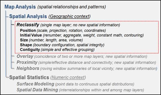
Figure 3. Reclassify operations involve reassigning
map values to reflect new information about existing map features.
For example, an initial
value based reclassification operation may involve the ranking or
weighting of qualitative map categories to generate a new map with quantitative
values. A map of soil types might be
assigned values that indicate the relative suitability of each soil type for
residential development. Quantitative
values also may be reclassified to yield new quantitative values. This might simply involve a specified
reordering of map categories (e.g., given a map of soil moisture content,
generate a map of suitability levels for plant growth). Or it could involve the application of a
generalized reclassifying function, such as “level slicing,” which splits a
continuous range of map categories values into discrete intervals (e.g.,
derivation of a contour map from a map of terrain elevation values).
Other quantitative
reclassification functions include a variety of arithmetic operations involving
map category values and a specified computed constant. Among these operations are addition,
subtraction, multiplication, division, exponentiation, maximization, minimization,
normalization and other scalar mathematical and statistical operators. For example, a map of topographic elevation
expressed in feet may be converted to meters by multiplying each map value by
3.28083 feet per meter.
Reclassification
operations also can relate to location-based, as well as purely thematic
attributes associated with a map. One
such characteristic is position. A map category represented by a single
“point” location (grid cell), for example, might be reclassified according to
its latitude and longitude. Similarly, a
line segment or areal feature could be reassigned values indicating its center
of gravity or orientation.
Another
location-based characteristic is size. In the case of map categories associated with
linear features or point locations, overall length or number of points may be
used as the basis for reclassifying those categories. Similarly, a map category associated with a
planar area may be reclassified according to its total acreage or the length of
its perimeter. For example, a map of
surface water might be reassigned values to indicate the areal extent of
individual lakes or length of stream channels.
The same sort of technique also might be used to deal with volume. Given
a map of depth to bottom for a group of lakes, for example, each lake might be
assigned a value indicating total water volume based on the areal extent of
each depth category.
In addition to value,
position and size of features, shape characteristics also may be
used as the basis for reclassifying map categories. Categories represented by point locations
have measurable shapes insofar as the set of points imply linear or areal forms
(e.g., just as stars imply constellations).
Shape characteristics associated with linear forms identify the patterns
formed by multiple line segments (e.g., dendritic stream pattern).
The primary shape characteristics associated with areal forms include
boundary convexity, nature of edge and topological genius.
Convexity and edge
address the “boundary configuration” of areal features. Convexity is the measure of the extent to
which an area is enclosed by its background relative to the extent to which the
area encloses its background. The
convexity index for a feature is computed by the ratio of its perimeter to its
area. The most regular configuration is
that of a circle which is convex everywhere along its boundary, and therefore,
not enclosed by the background at any point.
Comparison of a feature’s computed convexity with that of a circle of the
same area results in a standard measure of boundary regularity. The nature of the boundary at each edge
location can be used for a detailed description of boundary along a features
edge. At some locations the boundary
might be an entirely concave intrusion, whereas other locations might have
entirely convex protrusions. Depending
on the degree of “edginess,” each point can be assigned a value indicating the
actual boundary configuration at that location.
Topological genius
relates to the “spatial integrity” of an area.
A category that is broken into numerous fragments and/or containing
several interior holes indicates less spatial integrity than those without such
violations. The topological genius can
be summarized as the Euler number which is computed as the number of holes
within a feature less one short of the number of fragments which make up the
entire feature. An Euler number of zero
indicates features that are spatially balanced, whereas larger negative or
positive numbers indicate less spatial integrity.
A related operation,
termed “parceling,” characterizes contiguity. This procedure identifies individual clumps
of one or more locations having the same numerical value and which are
geographically contiguous (e.g., generation of a map identifying each lake as a
unique value from a generalized water map representing all lakes as a single
category).
This explicit use of shape/contiguity as analytic parameters is
unfamiliar to most Geotechnology users.
However, a non-quantitative consideration of landscape structure is
implicit in any visual assessment of mapped data. Particularly promising is the potential for
applying these techniques in areas of image classification and wildlife habitat
modeling. A map of forest stands, for
example, may be reclassified such that each stand is characterized according to
the relative amount of forest edge with respect to total acreage and frequency
of interior forest canopy gaps. Those
stands with a large portion of edge and a high frequency of gaps will generally
indicate better wildlife habitat for many species.
4.0 Spatial Analysis Procedures for Overlaying Maps
Operations for overlaying maps begin
to relate to the spatial, as well as the thematic nature of mapped data. The general class of overlay operations can
be characterized as “light-table gymnastics.”
The operations involves creation of a new map on which the value
assigned to each location or set of locations is a function of the independent
values associated with that location on two or more existing map layers. There are three basic approaches to
overlaying maps—Location-specific, and Region-wide
(figure 4).
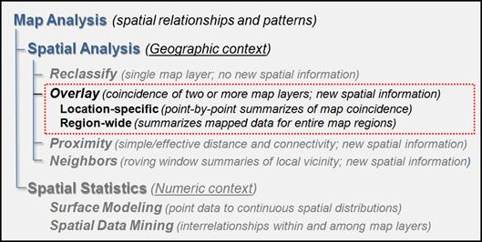
Figure 4.
Overlay operations involve characterizing the spatial coincidence of mapped
data.
In simple Location-specific
overlaying, the value assigned is a function of the point-by-point aligned
coincidence of existing maps. In
Region-wide compositing, values are assigned to entire thematic regions as a function
of the values associated with those regions contained on other map layers. Whereas the first overlay approach
conceptually involves the vertical spearing of a set of map layers, the latter
approach uses one layer to identify boundaries (termed the “template map”) for
which information is extracted in a horizontal summary fashion from the other
map layers (termed the “data maps”).
The most basic group of Location-specific
overlay operations computes new map values from those of existing map layers
according to the nature of the data being processed and the specific use of
that data within a modeling context.
Typical of many environmental analyses are those which involve the
manipulation of quantitative values to generate new quantitative values. Among these are the basic arithmetic
operations, such as addition, subtraction, multiplication, division, roots, and
exponentiation. For example, given maps
of assessed land values in 2000 and 2005, respectively, one might generate a
map showing the change in land values over that period as follows: (expressed
in MapCalcTM software syntax)
COMPUTE
2005_map MINUS 2000_map FOR Change_map
COMPUTE Change_map DIVIDEDBY 2005_map FOR Relative_Change_map
COMPUTE Relative_Change_map TIMES 100.0 FOR Percent_Change_map
Or as a
single map algebra equation:
CALCULATE
((2005_map - 2000_map)
/ 2005_map) * 100.0 FOR Percent_Change_map
Functions that relate to simple
statistical parameters such as maximum, minimum, median, mode, majority, standard
deviation, average, or weighted average also may be applied in this
manner. The type of data being
manipulated dictates the appropriateness of the mathematical or statistical
procedure used. For example, the
addition of qualitative maps such as soils and land use would result in
meaningless sums, as their numeric values have no mathematical
relationship. Other map overlay
techniques include several which may be used to process values that are either
quantitative or qualitative and generate values that may take either form. Among these are masking, comparison,
calculation of diversity and intersection.
Many of the more complex statistical
techniques comprising spatial statistics that will be discussed later involve
overlays where the inherent interdependence among spatial data is accounted for
in the continuous nature of the analysis frame.
These spatial data mining approaches treat each map as a “variable,”
each grid cell as a “case” and each value as an “observation” in an analogous
manner as non-spatial math/stat models.
A predictive statistical model, such as regression, can be evaluated for
each map location, resulting in a spatially continuous surface of predicted
values. The mapped predictions contain
additional information over traditional non-spatial procedures, such as direct
consideration of coincidence among regression variables and the ability to
locate areas of a given prediction level.
An entirely different approach to
overlaying maps involves Region-wide summarization of values. Rather than combining information on a
point-by-point basis, this group of operations summarizes the spatial
coincidence of entire categories of two or more maps. For example, the categories on a Cover_type map can be used to define areas over which the
coincident values on a Slope map are averaged.
The computed values of average slope are then used to renumber each of
the Cover_type categories. This processing can be implemented as:
(expressed in MapCalcTM
software syntax)
COMPOSITE Cover_type with Slope AVERAGE FOR Covertype_avgslope
Summary statistics that can be used in
this way include the total, average, maximum, minimum, median, mode, or
majority value; the standard deviation, variance, coefficient of variation or
diversity of values; and the correlation, deviation or uniqueness of particular
value combinations. For example, a map
indicating the proportion of undeveloped land within each of several districts
could be generated by superimposing a map of district boundaries on a map of
land use and computing the ratio of undeveloped land to the total area of each
district.
As with location-specific overlay
techniques, data types must be consistent with the summary procedure used. Also of concern is the order of data
processing. Operations such as addition
and multiplication are independent of the order of processing (termed “commutative operations”). However, other operations, such as
subtraction and division, yield different results depending on the order in
which a group of numbers is processed (termed “non-commutative operations”). This latter type of operations cannot be used
for region-wide summaries.
5.0 Spatial Analysis Procedures for
Establishing Proximity and Connectivity
Most geographic information systems contain
analytic capabilities for reclassifying and overlaying maps. The operations address the majority of
applications that parallel manual map analysis techniques. However to more fully integrate spatial
considerations into decision-making, new more advanced techniques are
available. The concept of distance
has been historically associated with the “shortest straight line distance
between two points.” While this measure
is both easily conceptualized and implemented with a ruler, it frequently is
insufficient in a decision-making context.
A straight line route might indicate
the distance “as the crow flies” but offers little information for a walking or
hitchhiking crow or other flightless creature.
Equally important to most travellers is to have the measurement of
distance expressed in more relevant terms, such as time or cost. The group of operations concerned with
distance, therefore, is best characterized as “rubber rulers.”
The basis of any system for
measurement of distance requires two components—a standard measurement unit and
a measurement procedure. The measurement unit used in most
computer-oriented systems is the “grid space” implied by the superimposing of
an imaginary uniform grid over geographic space (e.g., latitude/longitude or a custom
analysis grid). The distance from any
location to another is computed as the number of intervening grid spaces. The measurement
procedure always retains the requirement of “shortest” connection between
two points; however, the “straight line” requirement may be relaxed.
A frequently employed measurement
procedure involves expanding the concept of distance to one of proximity
(figure 5). Rather than sequentially
computing the distance between pairs of locations, concentric equidistant zones
are established around a location or set of locations. In effect, a map of proximity to a “target”
location is generated that indicates the shortest straight line distance to the
nearest target grid cell for each non-target location.
Within many application contexts, the
shortest route between two locations might not always be a straight line. And even if it is straight, the Euclidean
length of that line may not always reflect a meaningful measure of
distance. Rather, distance in these
applications is defined in terms of movement expressed as travel-time,
cost, or energy that may be consumed at rates that vary over time and
space. Distance modifying effects may be
expressed spatially as “barriers” located within the geographic space in which
the distance is being measured. Note
that this implies that distance is the result of some sort of movement over
that space and through those barriers.
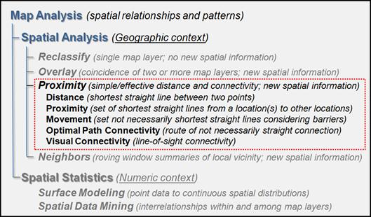
Figure 5.
Proximity operations involve measuring distance and connectivity among
map locations.
Two major types of barriers can be
identified as to how they affect the implied movement. “Absolute barriers” are those that completely
restrict movement and therefore imply an infinite distance between the points
they separate, unless a path around the barrier is available. A flowing river might be regarded as an
absolute barrier to a non-swimmer. To a
swimmer or boater, however, the same river might be regarded as a relative
rather than an absolute barrier.
“Relative barriers” are ones that are passable but only at a
cost/impedance which may be equated with an increase in effective distance.
For example, the hiking-time map from
a location can be calculated as set of concentric zones that vary in shape by
the relative influence various cover/slope categories for foot-travel
responding to the two types of barriers.
Open water such as lakes and large streams are treated as absolute barriers
that completely restrict hiking. The
land areas on the other hand, represent relative barriers to hiking which
indicate varied impedance to movement for each grid cell as a function of the
cover/slope conditions occurring at a location.
In a similar example, movement by
automobile might be effectively constrained to a network of roads (absolute
barriers) of varying speed limits (relative barriers) to generate a riding
travel-time map. Or from an even less
conventional perspective, effective-distance can be expressed in such terms as
accumulated cost of electric transmission line construction from an existing
trunk line to all other locations in a project area. The cost surface that is developed can be a
function of a variety of social and engineering factors, such as visual
exposure and adverse terrain, expressed as absolute and/or relative barriers.
The ability to move, whether
physically or abstractly, may vary as a function of the implied movement, as
well as the static conditions at a location.
One aspect of movement that may affect the ability of a barrier to
restrict that movement is direction. A
topographic incline, for example, will generally impede hikers differently
according to whether their movement is uphill, downhill or across slope. Another possible modifying factor is
accumulation. After hiking for a certain
distance, “mole-hills” tend to become disheartening mountains and movement
becomes more restricted for a tired hiker.
A third attribute of movement that may dynamically alter the effect of a
barrier is momentum or speed. If an old
car has to stop on steep hill, it might not be able to resume movement, whereas
if it were allowed to maintain its momentum (e.g., green light) it could easily
reach the top. Similarly, a highway
construction zone which reduces traffic speeds from 75 to 55 mph, for example,
would have little or no effect during rush hour when traffic already is moving
at a much slower speed.
Another distance related class of
operators is concerned with the nature of connectivity among locations. Fundamental to understanding these procedures
is the conceptualization of an “accumulation surface,” It the map value of a
simple proximity map from a location is used to indicate the third dimension of
a surface a uniform bowl would be depicted.
The surface configuration for an effective proximity map would have a
similar appearance; however, the bowl would be warped with numerous
ridges. Also, the nature of the surface
is such that it cannot contain saddle points (i.e., false bottoms). This “bowl-like topology” is characteristic
of all accumulation surfaces and can be conceptualized as a warped football
stadium with each successive ring of seats identifying concentric, equidistant
halos. The target or starting location(s)
is the lowest point and all other locations are assigned progressively larger
values of the shortest, but not necessarily straight distance from the
start. When viewed in perspective this
surface resembles a topographic surface with familiar valleys and hills. However in this case, the highlands indicate
areas that are effectively farther away from the starting location and there
can be no false bottoms along the ever-increasing gradient.
In the case of simple distance, the
delineation of paths, or “connectivity” lines, locate the shortest straight
line between any point on the surface and the starting point. Similarly, the steepest downhill path along
the accumulated surface of an effective distance respecting intervening
absolute/relative barriers identifies the shortest but not necessarily straight
path connecting any location to the starting point.
The procedure is analogous to the
steepest downhill path of water over a topographic surface to indicate surface
runoff. However the steepest path over a
proximity accumulation surface always ends at the starting/target location(s)
and effectively retraces the shortest route.
If an accumulation cost surface is considered, such as the cost for
transmission line construction, the minimum cost route will be located. If transmission line construction to a set of
dispersed locations were simultaneously considered, an “optimal path density”
map could be generated which identifies the number of individual optimal paths
passing through each location from the dispersed termini to a truck line start/target. Such a map would be valuable in locating
major feeder-lines (i.e., areas of high optimal path density) radiating from a
central trunk line.
Another connectivity operation
determines the narrowness of features.
The narrowness at each point within a map feature is defined as the
length of the shortest line segment that can be constructed through that point
to diametrically opposing edges of the feature (termed a “cord” in plane
geometry). The result of this processing
is a continuous map of features with lower values indicating relative narrow
locations within the feature. Panama,
for example, is at the narrowest point in the continental western
hemisphere. Or for a narrowness map of
forest stands, low values indicate interior locations with easy access to
edges.
The process of determining viewshed
involves establishing inter-visibility among locations. Locations forming the viewshed of an area are
connected by straight line-of-sight in three-dimensional space to the “viewer”
location, or set of viewers. Topographic
relief and surface objects form absolute barriers that preclude
connectivity. Atmospheric haze forms a
relative barrier and leaf on/off conditions can cause the vegetation canopy
result in different levels of opacity.
If multiple viewers are designated, locations within the viewshed may be
assigned a value indicating the number or density of visual connections.
6.0 Spatial Analysis Procedures for Depicting
Neighborhoods
The fourth and final group of spatial
analysis operations includes procedures that create a new map in which the
value assigned to a location is computed as a function of independent values
within a specified distance and direction around that location (i.e., its
geographic neighborhood). This general
class of operations can be conceptualized as “roving windows” moving throughout
a project area. The summary of
information within these windows can be based on the configuration of the surface (e.g., slope and aspect) or the statistical summary of thematic values
(figure 6).
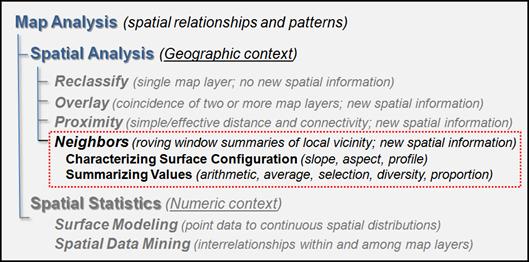
Figure 6.
Neighborhood operations involve characterizing mapped data within the
vicinity of map locations.
The initial step in characterizing
geographic neighborhoods is the establishment of
neighborhood membership. An
instantaneous neighborhood (roving window) is uniquely defined for each target
location as the set of points which lie within a specified distance and
direction around that location. The
roving window can assume different shapes based on geometric shape, direction
and distance. In most applications the
window has a uniform shape and orientation (e.g., a circle or square). However as noted in the previous section, the
distance may not necessarily be Euclidean nor symmetrical, such as a
neighborhood of “down-wind” locations within a quarter mile of a smelting
plant. Similarly, a neighborhood of the
“ten-minute drive” along a road network could be defined.
The summary of information within a
neighborhood may be based on the relative spatial configuration of values
that occur within the window. This is
true of the operations that measure topographic characteristics, such as slope,
aspect and profile from elevation values.
One such approach involves the “least-squares fit” of a plane to
adjacent elevation values. This process
is similar to fitting a linear regression line to a series of points expressed
in two-dimensional space. The
inclination of the plane denotes terrain slope and its orientation characterizes
the aspect/azimuth. The window is
successively shifted over the entire elevation map to produce a continuous
slope or aspect map.
Note that a “slope map” of any surface
represents the first derivative of that surface. For an elevation surface, slope depicts the
rate of change in elevation. For an
accumulation cost surface, its slope map represents the rate of change in cost
(i.e., a marginal cost map). For a
travel-time accumulation surface, its slope map indicates the relative change
in speed and its aspect map identifies the direction of optimal movement at
each location. Also, the slope map of an
existing topographic slope map (i.e., second derivative) will characterize
surface roughness (i.e., areas where slope is changing).
The creation of a “profile map” uses a
window defined as the three adjoining points along a straight line oriented in
a particular direction. Each set of
three values can be regarded as defining a cross-sectional profile of a small
portion of a surface. Each line is
successively evaluated for the set of windows along that line. This procedure may be conceptualized as
slicing a loaf of bread, then removing each slice and characterizing its
profile (as viewed from the side) in small segments along the upper edge. The center point of
each three member neighborhood is assigned a value indicating the profile form
at that location. The value assigned can
identify a fundamental profile class (e.g., inverted “V” shape indicative of a
ridge or peak) or it can identify the magnitude in degrees of the “skyward
angle” formed by the intersection of the two line segment of the profile. The result of this operation is a continuous
map of the surface’s profile as viewed from a specified direction. Depending on the resolution of an elevation
map, its profile map could be used to identify gullies or valleys running
east-west (i.e., “V” shape in multiple orthogonal profiles).
The other group of neighborhood
operations are those that summarize thematic values. Among the simplest of these involve the
calculation of summary statistics associated with the map values occurring
within each neighborhood. These
statistics may include the maximum income level, the minimum land value, the
diversity of vegetation within a
half-mile radius (or perhaps, a five-minute effective hiking distance) of each
target point.
Note that none of the neighborhood
characteristics described so far relate to the amount of area occupied by the
map categories within each roving window neighborhood. Similar techniques might be applied, however,
to characterize neighborhood values which are weighted according to spatial
extent. One might compute, for example,
the total land value within three miles of each target location on a per-acre
basis. This consideration of the size of
the neighborhood components also gives rise to several additional neighborhood
statistics including the majority value (i.e., the value associated with the
greatest proportion of the neighborhood area); the minority value (i.e., the
value associated with the smallest proportion); and the uniqueness (i.e., the
proportion of the neighborhood area associated the value occurring at the
target point itself).
Another locational attribute which may
be used to modify thematic summaries is the geographic distance from the target
location. While distance has already
been described as the basis for defining a neighborhood’s absolute limits, it
also may be used to define the relative weights of values within a neighborhood. Noise level, for example, might be measured
according to the inverse square of the distance from surrounding sources. The azimuthal relationship between
neighborhood location and the target point also may be used to weight the value
associated with that location. In
conjunction with distance weighting, this gives rise to a variety of spatial
sampling and interpolation techniques.
For example “weighted nearest-neighbors” interpolation of lake-bottom
temperature samples assigns a value to a non-sampled location as the
distance-weighted average temperature of a set of sampled points within its
vicinity.
7.0 Spatial Statistics Procedures for Surface
Modeling
Whereas spatial
analysis involves characterizing the “geographic context” of mapped data,
spatial statistics involves characterizing the “numerical relationships” of
mapped data. There are two basic classes
of spatial statistics: Surface Modeling
and Spatial Data Mining.
“Surface Modeling”
converts discrete point-sampled data into continuous map surfaces through density
analysis, spatial interpolation or map generalization techniques (figure
7). Density Analysis establishes a
surface by summarizing the point values within a specified distance of each map
location. For example, a “customer
density surface” can be derived from geo-coded sales data to depict the peaks
and valleys of customer concentrations throughout a city by simply counting the
number of point values within a specified distance from each location.
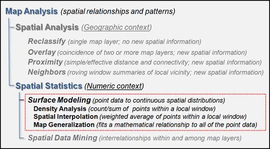
Figure 7.
Surface Modelling operations involve creating continuous spatial
distributions from point sampled data.
The procedure is analogous to poking pins on a map at each customer location and visually interpreting
the pattern of customer clusters.
However the result is a quantitative representation of customer data
expressed over continuous geographic space.
If the point values are summed a “total sales surface” is created (e.g.
total sales per square mile). If the
values are averaged, an “average sales surface” is created.
The subtle peaks
(lots of customers/sales nearby) and valleys (few customers/sales nearby) form
a continuous “spatial distribution” that is conceptually similar to a
“numerical distribution” that serves as the foundation of traditional
statistics. In this instance, three
dimensions are used to characterize the data’s dispersion—X and Y coordinates
to position the data in geographic space and a Z coordinate to indicate the
relative magnitude of the variable (i.e., number of customers or total/average
sales). From this perspective, surface
modeling is analogous to fitting a density function, such as a standard normal
curve, in traditional statistics. It
translates discrete point samples into a continuous three-dimensional surface
that characterizes both the numeric and geographic distribution of the data.
Spatial Interpolation is similar to density analysis as it utilizes spatial patterns in a
point sampled data set to generate a continuous map surface. However spatial interpolation seeks to
estimate map values instead of simply summarizing them. Conceptually it “maps the variance” in a set
of samples by using geographic position to help explain the differences in the
sample values. Traditional statistics
reduces a set of sample values to a single central tendency value (e.g.,
average) and a metric of data dispersion about the typical estimate (e.g.,
standard deviation). In geographic space
this scalar estimate translates into a flat plane implying that the average is
assumed everywhere, plus or minus the data dispersion. However, non-spatial statistics does not
suggest where estimates might be larger or where they might be smaller than the
typical estimate. The explicit spatial
distribution, on the other hand, seeks to estimate values at every location
based on the spatial pattern inherent in the sample set.
All spatial
interpolation techniques establish a "roving window" that—
- moves to a grid location in a project area (analysis
frame),
- calculates a weighted average of the
point samples around it (roving window),
- assigns the weighted average to the center cell of the
window, and then
- moves to the
next grid location.
The extent of spatial
interpolation’s roving window (both size and shape) affects the result,
regardless of the summary technique. In general, a large window capturing
a larger number of values tends to smooth the data. A smaller window
tends to result in a rougher surface with more abrupt transitions.
Three factors affect
the window's extent: its reach, the number of samples, and balancing. The reach,
or search radius, sets a limit on how far the computer will go in collecting
data values. The number of
samples establishes how many data values should be used. If there
is more than the specified number of values within a specified reach, the
computer just uses the closest ones. If there are not enough values, it
uses all that it can find within the reach.
Balancing of the data
attempts to eliminate directional bias by ensuring that the values are selected
in all directions around window's center.
The weighted averaging procedure is
what determines the different types of spatial interpolation techniques. The Inverse Distance Weighted (IDW) algorithm
first uses the Pythagorean Theorem to calculate the Distance from a
Grid Location to each of the data samples within the summary window. Then the distances are converted to weights
that are inversely proportional to the distance (e.g., 1/D2),
effectively making more distant locations less influential. The sample values are multiplied by their
corresponding computed weights and the “sum of the products” is divided by the
“sum of the weights” to calculate a weighted average estimate. The estimate is assigned to center cell
location and the process is repeated for all map locations.
The inverse distance
procedure used a fixed, geometric-based method to estimate map values at
locations that were not sampled. An
alternative algorithm, termed Krigging, an advanced spatial statistics
technique that uses data trends in the sample data to determine the weights for
averaging. Other roving window-based
techniques, such as Natural Neighbor,
Minimum Curvature, Radial Basis Function and Modified Shepard’s
Method, use different techniques to weight the samples within the roving
window.
Map Generalization, on the other hand, involves two additional
surface modeling approaches that do not use a roving window: Polynomial Surface
Fitting and Geometric Facets. Both approaches consider the
entire set of sample points in deriving a continuous map surface. In Polynomial Surface Fitting the degree of
the polynomial equation determines the configuration of the final surface. A first degree polynomial fits a plane to the
data such that the deviations from the plane to the data are minimized. The result is a tilted plane that indicates
the general trend in the data. As higher
degree polynomials are used the plane is allowed to bend and warp to better fit
the data.
In Geometric Facets interpolation the procedure
determines the optimal set of
triangles connecting all the points. A Triangulated Irregular Network (TIN) forms a tessellated
model based on triangles in which the vertices of the triangles form irregularly
spaced nodes that allows dense information in areas where the implied surface
is complex, and sparse information in simpler or more homogeneous areas.
While there numerous techniques for characterizing the spatial distribution inherent in a set of
point-sampled data there are three critical conditions that govern the results:
data type, sampling intensity and sampling pattern. The data must be continuous in both numeric
space (interval or ratio) and geographic space (isopleth). Also, the number of samples must be large
enough and well-dispersed across the project area to capture inherent
geographic pattern in the data.
8.0 Spatial Statistics Procedures for Spatial
Data Mining
Surface modeling
establishes the continuous spatial distribution as map layers in map
stack. “Spatial Data Mining” is the
process of characterizing numerical interrelationships among the mapped data
layers through three basic approaches: descriptive, predictive and prescriptive
statistics (figure 8).
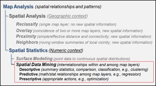
Figure 8.
Spatial Data Mining operations involve characterizing numerical patterns
and relationships among mapped data.
Basic descriptive statistics involve
calculating the mode, median, mean, range, variance, standard
deviation, coefficient of variation and other scalar metrics for all or part of
individual maps or a map stack. For
example, region-wide overlay may be used to calculate the average parts per
million by administrative districts for a spatially interpolated map surface of
lead concentrations based on soil samples.
A computed coefficient of variation may be included to establish the
amount of data dispersion within each district. Or the mean of a weekly time
series of airborne lead concentration over a city could be averaged to identify
seasonal averages (location-specific overlay).
In a similar manner,
two of the weekly maps could be compared by simply subtracting them for the
absolute difference or computing the percent change. Another comparison technique could be a Paired t-test of the two maps to determine if
there is an overall significant difference in the two sets of map values.
Map classification can be simply
generalizing a continuous range of map values through contouring or employing
sophisticated techniques like the supervised (e.g., maximum likelihood
classifier) and unsupervised (e.g., clustering classifier) approaches used in
remote sensing to distinguish land cover groups from map stacks of satellite
spectral data. These approaches utilize
standard multivariate statistics to assess the “data space distance” among
individual data patterns within the map stack.
If the data distance is small the map value patterns are similar and can
be grouped; if the data distance is large separate thematic classes are
indicated.
Predictive statistics establish a spatial relationship among a mapped variable and its
driving variables, such as sales and demographic data or crop yield and soil
nutrient maps. For example, linear
regression can be used to derive an equation that relates crop yield (termed
the “dependent” mapped variable) to phosphorous, potassium, nitrogen, pH,
organic matter and other plant growth factors (termed the “independent” mapped
variables).
Once a statistical
relationship is established prescriptive statistics it can be
used to generate a “prescription map.”
In the crop yield example, the equation can be used to predict yield
given existing soil nutrient levels and then analyzed to generate a
prescription map that identifies the optimal fertilizer application needed at
each map location considering the current cost of fertilizer and the estimated
market price of the increased yield expected.
Another application might derive a regression relationship among product
sales (dependent) and demographics (independent) through a test marketing
project and then spatially apply the relationship to demographic data in
another city to predict sales. The
prediction map could be used to derive prescription maps of locations requiring
infrastructure upgrade or marketing investment prior to product
introduction.
For the most part, spatial data mining
employs traditional data analysis techniques.
What discriminates it is its data structure, organization and ability to
infuse spatial considerations into data analysis. The keystone concept is the analysis frame of grid
cells that provides a quantitative representation of the continuous spatial
distributions of mapped variables. Also
this structure serves as the primary key for linking spatial and non-spatial
data sets, such as customer records, or crime incidence, or disease
outbreak. With spatial data mining,
geographic patterns and relationships within and among map layers are
explicitly characterized and utilized in the numerical analyses.
9.0 Procedures for Communicating Model Logic
The preceding sections have developed
a typology of fundamental map analysis procedures and described a set of
spatial analysis (reclassify, overlay distance and neighbours) and spatial
statistics (surface modeling and spatial data mining) operations common to
broad range of techniques for analyzing mapped data. By systematically organizing these primitive
operations, the basis for a generalized GIS modeling approach is
identified. This approach accommodates a
variety of analytical procedures in a common, flexible and intuitive manner
that is analogous to the mathematical of conventional algebra.
As an example of some of the ways in which
fundamental map analysis operations may be combined to perform more complex
analyses, consider the GIS model outlined in figure 9. Note the format used in the schematic in
which “boxes” represent encoded and derived maps and “lines” represent primitive
map analysis operations. The flowchart
structure indicates the logical sequencing of operations on the mapped data that progresses to the final map. The simplified model depicts the location of
an optimal corridor for a highway considering only two criteria: an engineering
concern to avoid steep slopes, and a social concern to avoid visual
exposure.
It is important to note that the model
flowchart is organized such that the “rows” identify the processing of the
criteria, while the “columns” identify increasing levels of abstraction from
physical base maps to conceptual suitability maps representing relative
“goodness,” and then to a map of the optimized best route.
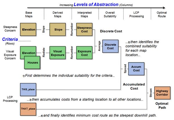
Figure 9. GIS
modeling logic can be expressed as a flowchart of processing with “boxes”
representing existing/derived maps and “lines” representing map analysis
operations. (MapCalcTM
software commands indicated)
Given a grid map layer of topographic
Elevation values and a map of Houses, the model allocates a least-cost highway
alignment between two predetermined locations.
Cost is not measured in dollars, but in terms of relative
suitability. The top-left portion of the
model develops a “discrete cost surface” (identified as the Discrete Cost map)
in which each location is assigned a relative cost based on the particular
steepness/exposure combination occurring at that location. For example, those areas that are flat and
not visible from houses would be assigned low cost values; whereas areas on
steep slopes and visually exposed would be assigned high values. This discrete cost surface is used as a map
of relative barriers for establishing an accumulated cost surface (Accum Cost) from one of the two termini to all other
locations (THISplace). The final step locates the other terminus (THATplace) on the accumulated cost surface and identifies
the minimum cost route as the steepest downhill path along the surface from
that point to the bottom (i.e., the other end point).
The highway corridor application is
representative of a “suitability model” where geographic considerations are
translated into preferences for the location of an activity or facility. A “physical model,” on the other hand,
characterizes a spatial process, such as overland water movement and subsequent
sediment loading estimates to a stream channel.
A “statistical model” establishes numerical relationships, such as crop
yield throughout a farmer’s field based on the geographic distribution of soil
nutrients like phosphorous, potassium and nitrogen. All three types of models
use a common set of primitive map analysis operations in a cyclical manner to
express solutions to complex spatial problems in a logical framework that is
easily communicated.
10.0 Impact of Spatial Reasoning and Dialog on
the Future of Geotechnology
In addition to the benefits of
efficient data management and automated mapping engrained in GIS technology,
the map analysis modeling structure has several additional advantages. Foremost among these is the capacity of
“dynamic simulation” (i.e., spatial “what if” analysis). For example, the highway corridor model
described in the previous section could be executed for several different
interpretations of engineering and social criteria. What if the terrain steepness is more
important, or what if the visual exposure is twice as important? Where does the least cost route change? Or just as important, where does it not
change? From this perspective the model
“replies” to user inquiries, rather than “answering” them with a single static
map rendering—the processing provides information for decision-making, rather
than tacit decisions.
Another advantage to map analysis and
modeling is its flexibility. New
considerations can be added easily and existing ones refined. For example, the non-avoidance of open water
bodies in the highway model is a major engineering oversight. In its current form the model favors construction on lakes, as they are flat and
frequently hidden from view. This new
requirement can be incorporated readily by identifying open water bodies as
absolute barriers (i.e., infinite cost) when constructing the accumulation cost
surface. The result will be routing of
the minimal cost path around these areas of extreme cost.
GIS modeling also provides an
effective structure for communicating both specific application considerations
and fundamental principles. The
flowchart structure provides a succinct format for communicating the processing
considerations of specific applications.
Model logic, assumptions and relationships are readily apparent in the
box and line schematic of processing flow.
Management of land always has required
spatial information as its cornerstone process.
Physical description of a management unit allows the conceptualization
of its potential usefulness and constrains the list of possible management
practices. Once a decision has been made
and a plan implemented, additional spatial information is needed to evaluate
its effectiveness. This strong
allegiance between spatial information and effective management policy will
become increasing important due to the exploding complexity of issues our world’s
communities. The spatial reasoning
ingrained in GIS modeling provides the ability “to truly think with maps” and
is poised to take Geotechnology to the next level.
Acknowledgments
The basic framework described in this
paper was developed through collaborative efforts with C. Dana Tomlin in the
early 1980’s in the development of a workbook and numerous workshop
presentations on “Geographic Information Analysis” by J. K. Berry and C. D.
Tomlin, Yale School of Forestry and Environmental Studies, New Haven,
Connecticut, 206 pages.
References
-
Berry, J.K. 1985. Computer-assisted map analysis: fundamental
techniques. National Association of
Computer Graphics, Computer Graphics ’85 Conference Proceedings, pgs. 112-130.
-
Berry, J.K. 2009. What’s
in a name? GeoWorld, Beyond Mapping column, March, Vol
22, No. 3, pp 12-13.
-
Gewin, V.
2004. Mapping opportunities. Nature 427, 376-377 (22 January 2004).
-
Tomlin, C.D. and J.K. Berry, 1979. A
mathematical structure for cartographic modeling in environmental analysis. American Congress on Surveying and Mapping,
39th Symposium Proceedings, pgs. 269-283.
-
Tomlin, C.D., 1990. Geographic
Information Systems and Cartographic Modeling, Prentice Hall publishers, Englewood Cliffs, New Jersey.
Further
Reading
Two primary resources support further
study of the map analysis operations and GIS modeling framework described in
this paper: the text book Map Analysis and the online book Beyond
Mapping III. Table 1 below serves as a cross-listing of the sections in
this paper to topics in the referenced resources containing extended discussion
and hands-on experience with the concepts, procedures and techniques
presented.
In addition, Chapter 29, “GIS Modeling and Analysis,” by J.K.
Berry in the Manual of Geographic
Information Systems, American Society for Photogrammetry &
Remote Sensing (ASPRS, in press) contains nearly 100 pages and over 50
illustrations expanding on the framework and material presented in this paper.
Table 1. Cross-listing to Further Reading Resources
|
The Map Analysis text is a
collection of selected works from of Joseph K. Berry’s popular “Beyond
Mapping” columns published in GeoWorld magazine from 1996 through 2006. In this compilation Berry develops a
structured view of the important concepts, considerations and procedures
involved in grid-based map analysis and modeling. The companion CD contains further readings
and MapCalcTM software for hands-on
experience with the material. Map Analysis:
Understanding Spatial Patterns and Relationships by Joseph K. Berry, 2007, GeoTec Media
Publishers, 224 pages, 105 figures; US$45 plus shipping and
handling. For more information and
ordering, see www.geoplace.com/books/mapanalysis/. |
||
|
The Beyond Mapping III online book
is posted at www.innovativegis.com/basis/MapAnalysis/ and
contains 28 topics on map analysis and GIS modeling. Over 350 pages and nearly 200 illustrations
with hyperlinks for viewing figures in high resolution and permission granted
for free use of the materials for educational purposes. |
||
|
|
||
|
Section in this Paper |
Map Analysis |
Beyond Mapping III |
|
1.0 Introduction |
Foreword,
Preface, Introduction |
Introduction |
|
2.0 Nature of Discrete versus Continuous
Mapped Data |
Topic 1 Data Structure
Implications Topic 2 Fundamental Map
Analysis Approaches |
Topic 1 Object-Oriented Technology Topic 7 Linking Data Space and Geographic Space Topic
18 Understanding Grid-based Data |
|
3.0 Spatial Analysis Procedures for
Reclassifying Maps |
Topic 3 Basic Techniques in
Spatial Analysis |
Topic
22 Reclassifying and Overlaying Maps |
|
4.0 Spatial Analysis Procedures for
Overlaying Maps |
Topic 3 Basic
Techniques in Spatial Analysis |
Topic
22 Reclassifying and Overlaying Maps |
|
5.0 Spatial Analysis Procedures for
Establishing Proximity and Connectivity |
Topic 4 Calculating
Effective Distance Topic 5 Calculating Visual
Exposure |
Topic 5 Analyzing Accumulation Surfaces Topic 6 Analyzing In-Store Shopping Patterns Topic 13 Creating Variable-Width Buffers Topic 14 Deriving and Using Travel-Time Maps Topic 15 Deriving and Using Visual Exposure Maps Topic 17 Applying Surface Analysis Topic
19 Routing and Optimal Paths Topic
20 Surface Flow Modeling Topic
25 Calculating Effective Distance |
|
6.0 Spatial Analysis Procedures for Depicting
Neighborhoods |
Topic 6 Summarizing
Neighbors |
Topic 9 Analyzing Landscape Patterns Topic 11 Characterizing Micro Terrain Features Topic
26 Assessing Spatially-Defined Neighborhoods |
|
7.0 Spatial Statistics Procedures for Surface
Modeling |
Topic 9 Basic Techniques in
Spatial Statistics |
Topic 2 Spatial Interpolation Procedures and Assessment Topic 3 Considerations in Sampling Design Topic 8 Investigating Spatial Dependency Topic
24 Overview of Spatial Analysis and Statistics |
|
8.0 Spatial Statistics Procedures for Spatial
Data Mining |
Topic 10 Spatial Data Mining |
Topic 10 Analyzing Map Similarity and Zoning Topic 16 Characterizing Patterns and Relationships Topic
28 Spatial Data Mining in Geo-business |
|
9.0 Procedures for Communicating Model Logic |
Topic 7 Basic Spatial
Modeling Approaches Topic 8 Spatial Modeling
Example |
Topic
23 Suitability Modeling |
|
10.0 Impact of Spatial Reasoning and Dialog on
the Future of Geotechnology |
Epilogue |
Topic 4 Where Is Topic 12 Landscape Visualization Topic
21 Human Dimensions of GIS Topic
27 GIS Evolution and Future Trends Epilogue |
In addition, a book chapter expanding
on the framework described in this paper is posted online. “
Finally, the Beyond Mapping
Compilation Series by Joseph K. Berry is a collection of Beyond Mapping columns appearing
in GeoWorld (formally
GIS World) magazine from March
1989 through December 2013 that contains nearly 1000 pages and more than 750 figures providing
a comprehensive and longitudinal perspective of the underlying concepts,
considerations, issues and evolutionary development of modern geotechnology is posted at www.innovativegis.com/basis/BeyondMappingSeries.
Selected
Additional Resources on grid-based map analysis include:
-
DeMers, M. N. 2001.
GIS Modeling in Raster, John Wiley & Sons, Ltd. Publisher,
West Sussex, England.
-
de Smith, M. J., M.F. Goodchild, and P.A Longley
2007. Geospatial Analysis: A Comprehensive Guide to Principles, Techniques
and Software Tools, Troubador Publishing Ltd.,
Leicester, UK.
-
Fotheringham, S. and P. Rogerson (editors) 1994. Spatial Analysis and GIS (Technical
Issues in Geographic Information Systems) CRC Press, Florida.
-
Fotheringham, S. and
P. Rogerson (editors) 2009. Handbook of Spatial Analysis, Sage
Publications Ltd. Publisher.
-
Longley, P. A. and M. Batty (editors)
1997. Spatial Analysis: Modelling in
a GIS Environment, John Wiley & Sons, Ltd. Publisher, West Sussex,
England.
-
Longley, P. A., M. F. Goodchild,
D.J Maguire and D.W. Rhind 2001. Geographic Information Systems and Science,
John Wiley & Sons, Ltd. Publisher, West Sussex, England.
-
Longley, P. A. and M. Batty (editors) 2003. Advanced Spatial Analysis: The CASA Book of
GIS, ESRI Press, Redlands, California.
-
Maguire D. and M. Batty (editors) 2005. GIS, Spatial Analysis and Modeling,
ESRI Press, Redlands, California.
-
Mitchell, A. 1999. The ESRI Guide to GIS Analysis Volume 1: Geographic
Patterns & Relationships, ESRI Press, Redlands, California.
-
Mitchell, A. 2005. The ESRI Guide to GIS Analysis: Volume 2:
Spatial Measurements and Statistics, ESRI Press, Redlands, California.
_____________________________________