Beyond Mapping III
|
Map
Analysis book with companion CD-ROM for hands-on exercises and further reading |
Traditional Approaches Can’t Characterize Overland Flow — describes
the basic considerations in overland flow
Constructing Realistic Downhill Flows Proves
Difficult — discusses
procedures for characterizing path, sheet, horizontal and fill flows
Use Available Tools to Calculate Flow Time and
Quantity — discusses
procedures for tracking flow time and quantity
Migration Modeling Determines Spill Effect — describes
procedures for assessing overland and channel flow impacts
Author’s
Notes: The figures in this topic use MapCalcTM
software. An educational CD with online
text, exercises and databases for “hands-on” experience in these and other grid-based
analysis procedures is available for US$21.95 plus shipping and handling (www.farmgis.com/products/software/mapcalc/
).
<Click
here> right-click to download a printer-friendly version of this topic
(.pdf).
(Back to the Table of Contents)
______________________________
Traditional Approaches Can’t Characterize
(GeoWorld, November 2003, pg. 20-21)
Common sense suggests that “water flows downhill” however
the corollary is “…but not always the same way.” Similarly, overland flow modeling in a
The pipeline industry has been mandated to determine the
flows that would occur if a release were to happen at any location along a
pipeline route—that could be from
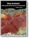
Figure 1 outlines the major steps of an Overland Flow model for tracking potential spill migration. The first step positions a pipeline on an elevation surface. Then a spill point along the pipeline is identified and its overland flow path (downhill) identified. In an iterative fashion, successive spill points and their paths are identified.
High Consequence Areas (HCAs) are delineated on maps prepared by the Office of Pipeline Safety. These include areas such as high population concentrations, drinking water supplies and critical ecological zones. The HCAs impacted by individual spills are identified and recorded in a database table. The final step identifies where paths enter streams or lakes and passes the information to a Channel Flow module (subject for future discussion).
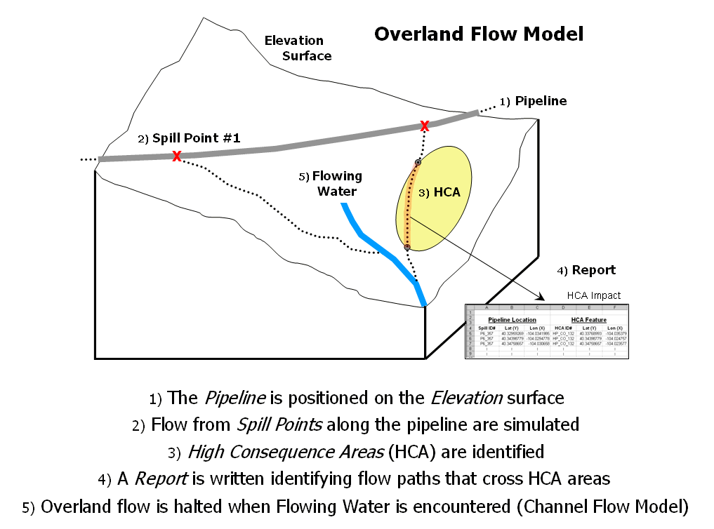
Figure 1. Spill mitigation for pipelines identifies high consequence areas that could be impacted if a spill occurs anywhere along a pipeline.
The centerline of the pipeline usually is stored as a series
of vector lines in an existing corporate database. USGS’s National Elevation Data (NED) data set
is available for the entire
Developing a realistic model of overland flow is just as challenging. Real world flows are complex and need to consider differences in terrain slopes, product types and intervening conditions. In addition, information on the timing and quantity of flow as the path progresses is invaluable in spill migration planning.
The top portion of figure 2 shows the spill patterns for three different locations along a pipeline assuming perfectly flat terrain. The jagged edges of the patterns result from approximating circles through grid-based proximity analysis. The progressively larger rings are analogous to slowly dripping coffee on your desk …first a small spill, then growing a little larger and a little larger, etc.
Now let’s add a bit reality. The middle series of maps identify the elevation surface for the area. The insets on the right show the downhill locations from each of the three spill points. The colored bands identify increasing distance with red tones identifying locations close to a spill.
A final bit of reality recognizes that not all downhill locations affect flow in the same manner. The Flow Impedance map at the lower left incorporates the effects of terrain slope on flow velocity. In flat or gently sloped areas (<2% slope), flow is gradual and can take several minutes to traverse a 30 meter cell. In steep areas, on the other hand, the same distance can take far less than a minute.
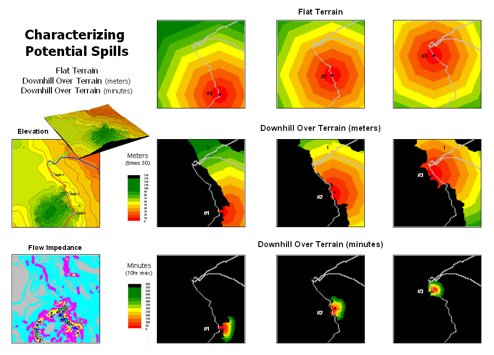
Figure 2. Overland flow can be
characterized as both distance traveled
and elapsed time.
This information is taken into account to generate maps at the bottom-right of figure 2. The results show a downhill flow “reach” of several hours for the three simulated spill points. Note that most of the flow occurs on very gentle slopes (cyan and light grey on the Flow Impedance map) so progress isn’t very fast or far.
Figure 3 depicts the processing flowchart and results for simulating overland flow from all locations defining the pipeline. The procedure is analogous to tossing a stick shaped like the pipeline into a pond. Ripples move outward indicating increasing distance. However in this instance, the waves can’t go uphill and the shortest elapsed time to reach any location is calculated.
The grey areas on the resultant map identify uphill locations (infinitely far away). The red tones identify areas that are relatively close to the pipeline. They progress to green tones identifying locations that are several hours away.
Figure 3. Effective downhill proximity from a pipeline can be mapped
as a variable-width buffer.
As we’ll see in next month’s column, things get even more complex as various terrain conditions (path, sheet, flat flow and pooling) and product properties (viscosity, release amount, etc.) come into play. The bottom line is that the traditional approach of choosing just the steepest downhill path for characterizing overland flow doesn’t hold water.
Constructing Realistic
Downhill Flows Proves Difficult
(GeoWorld, December 2003, pg. 20-21)
The instinct of a herd of rain drops is unwavering. As soon as they hit the ground they start running downhill as fast as they can. But not all downhill options are the same. Some slopes are extremely steep and call the raindrops like a siren. Other choices are fairly flat and the herd tends to spread out. Depressions in the terrain cause them to backup and pool until they can break over the lip and start running downhill again.
In overland flow modeling these conditions are termed path, sheet, flat and pooling flows. Figure 1 depicts two downhill paths over a terrain surface that is displayed in its raw form as grid cells raised to the relative height of their elevation values. A starting point on the surface is identified and the computer simulates the downhill route.
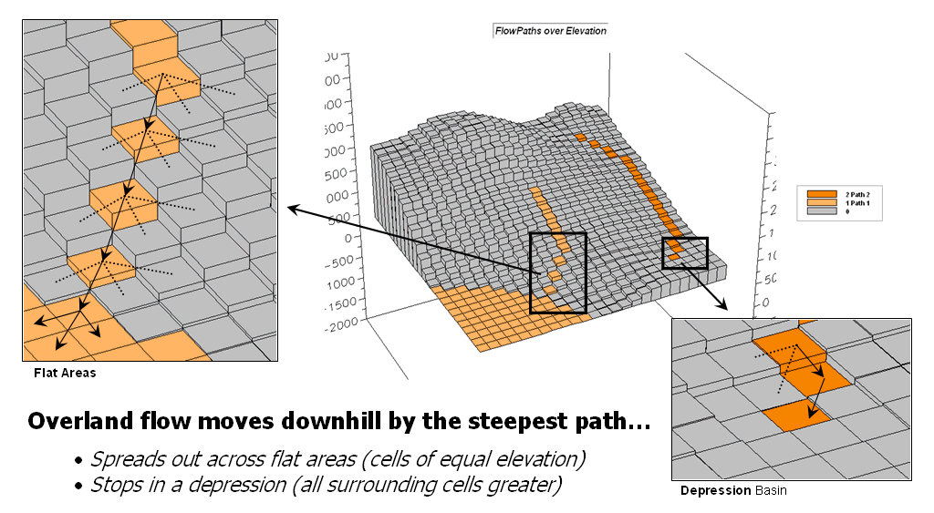
Figure 1. Surface flow takes the
steepest downhill path whenever possible
but spreads out in flat areas and pools in depressions.
As shown in the enlarged inset on the right, a location along the path could potentially flow to any of its neighboring cells. Uphill possibilities with larger elevation values are immediately eliminated (educated raindrops). The steepest downhill step is determined and path flow moves to that location. The process is repeated over and over to identify the steps along the steepest downhill path.
This procedure works nicely until reality sets in. What happens when a flat areas are encountered? No longer is there a single steepest downhill step because all surrounding elevation values are equal or larger. Obviously the flow doesn’t stop; it simply spreads out into the flat area. In this instance the algorithm must follow the raindrop’s lead and incorporate code that continues spreading as shown in the figure. The “steepest downhill path, then stop” approach isn’t sufficient. Nor is a path that simply shoots a straight line across the flat area a realistic solution.
However, realistic flow modeling is even more subtle than that. Areas of very gentle slope but not perfectly flat tend to exhibit sheet flow and spread out to all of the slight downhill locations. Figure 2 depicts the different conditions for path, sheet and flat flow.
The upper-left inset (a) shows the steepest downhill path in areas of steep terrain. Inset (b) shows the sheet flow widening to all downhill locations when inclination is slight.
Inset (c) depicts the flow going in all directions on perfectly flat terrain. As an empirical test, the next time you are doing the dishes hold a cutting board under the faucet and watch the water pattern change as you tilt the board from horizontal to steeper inclinations—flat, sheet then increasingly narrow path flows.
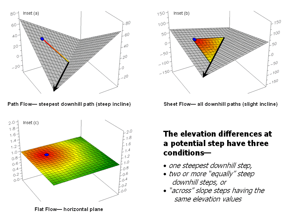
Figure 2. Surface inclination
and liquid type determine the type
of surface flow—path, sheet or flat.
Incorporating sheet flow into the algorithm inserts a test that determines if the steepest downhill step is less than a specified angle—if so, then steps to all of the downhill locations are taken. Another confounding condition occurs when there are equally steep downhill possibilities. In this instance both steps are taken and the flow path broadens or splits.
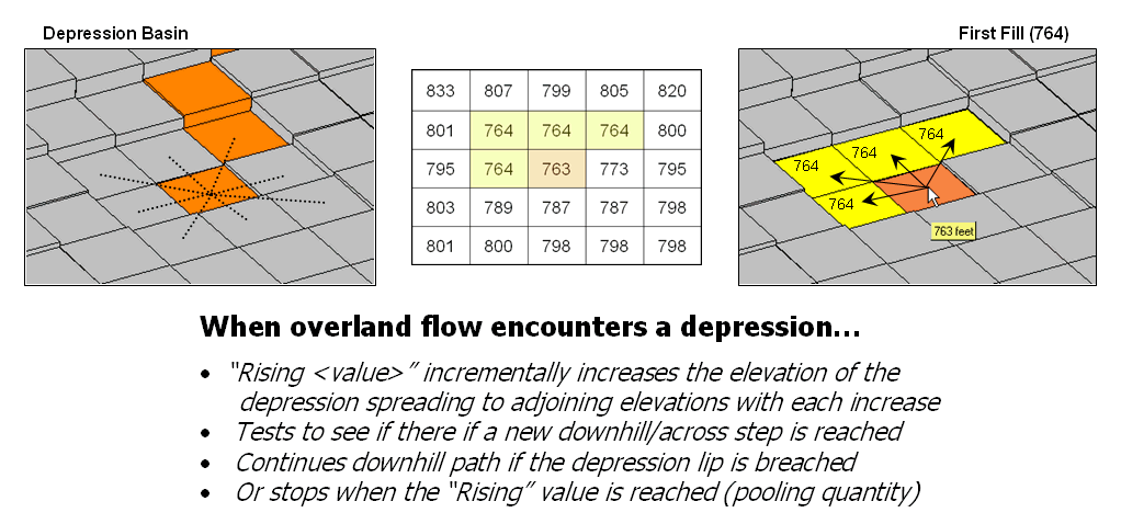
Figure 3. Pooling of surface
flow occurs when depressions are encountered.
By far the trickiest flow for a computer to simulate is pooling. Figure 3 shows a path that seemingly stops when it reaches a depression. In this instance, all of the elevation values around it are larger and there are no downhill or across steps to take. As more and more raindrops backup in confusion they start filling the depression. When they reach the height of the smallest elevation surrounding them they flow into it.
That is the same procedure the computer algorithm uses. It searches the neighboring cells for the smallest elevation, fills to that level, and then steps to that location. The procedure of filling and stepping is repeated until the lip of the depression is breached and flow downhill can resume.
Another possibility is that the quantity of flowing liquid is exhausted and the path is terminated at a pooling depth that fails to completely fill the depression. The idea of tracking flow quantity, as well as elapsed time, along a flow path is an important one, particularly when modeling pipeline spill migration. That discussion is reserved for next month.
Use Available Tools to
Calculate Flow Time and Quantity
(GeoWorld, January 2004, pg. 18-19)
The last couple of sections have investigated overland flow
modeling with a
A fourth type of flow—pooling—occurs when a depression is encountered. In this instance flow continues rising until it fills the depression and can proceed further downhill or the available quantity of liquid is trapped.
The introduction of flow quantity and timing are important concepts in modeling pipeline spill events. It’s common sense that a 100 barrel release won’t travel as far as a 1000 barrel release from the same location. Similarly, a “gooey” liquid takes longer to flow over a given distance than a “watery” one.
So how does the computer track retained quantity and elapsed time along a spill path? Several factors come into play involving cell size, properties of the liquid, terrain configuration and intervening conditions. Viscosity and specific gravity determine the “gooeyness” of flowing liquid and the effective depth of the flow.
This, plus the steepness of the terrain, determines the amount of liquid that is retained on the surface at each location. Add an infiltration factor for seepage into the soil and you have a fairly robust set of flow equations. In mathematical terms, this relationship can be generalized as—
Quantity Retained = fn [cellsize,
flow depth, slope angle, soil permeability]
Flow Velocity = fn [gravitational
constant, viscosity, specific gravity, flow depth, slope angle]
Implementing the cascading flow in a
In terms of pipeline spill mitigation, the quantities of jet fuel (thin) or crude oil (thick) that are retained along a flow path can be dramatically different. Equally striking are the differences in quantities that seep into dissimilar soil types. Also, if the spill occurs when the soil is saturated or frozen, infiltration will be minimal with nearly all of the quantity continuing along the path. Coding for all of these contingencies is what makes a spatially-specific model particularly challenging.
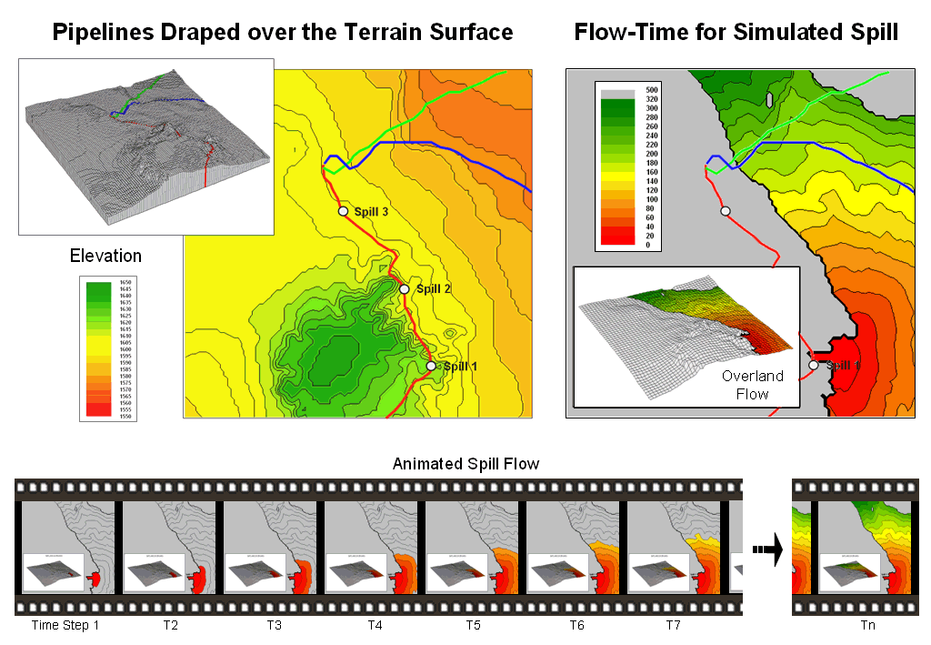
Figure 1. Overland flow is
calculated as a series of time steps traveling downhill over an elevation
surface.
Figure 1 shows the overland flow from a simulated spill. It is a conservative estimate as the simulation assumes sheet/flat flow at minimal inclinations, no soil infiltration and an unlimited quantity of liquid. In addition, the flow is measured in units of time by successively adding the time to cross each grid cell (time= cell length / flow velocity) as the flow proceeds.
The lower inset in the figure depicts an animation series of flow progress in 20 minute time steps. Note that the simulated release starts in relatively steep terrain of about 6 percent but quickly fans out as more gentle terrain is encountered. The maximum extent within the project area occurs at the northern portion and is reached in a little over five hours.
Figure 2 compares the flow times for two different liquid
types over the same terrain.
In Mr. Wizard terms, it means if you pour a cup of water on a tilted cutting board most of it runs off almost instantly. However, if you pour a cup of honey on the same board it takes much longer to flow down and a relatively larger portion sticks to the board.
The quantity and velocity equations quantitatively account for these common sense characteristics of overland flow. While neither the equations nor the data are perfect, the extension of the cutting board example to the grid cell element provides a radically new approach to modeling overland flow.
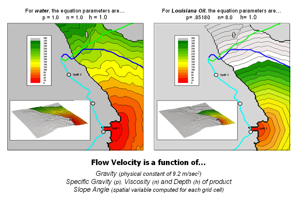
Figure 2. Flow velocity is dependent on the type of liquid and the steepness of the terrain.
Research into the equations has been ongoing for decades. However, in real-world applications the effects of slope angle could not be adequately modeled until the advent of map analysis tools and extensive data. Today, we have seamless elevation data for the contiguous fifty states (National Elevation Dataset) that can be purchased for about $1500. The pieces are in place—equations, technology and data—for realistic modeling of overland flow. As we’ll see next month the same holds for modeling channel flow.
Migration Modeling Determines Spill Effect
(GeoWorld, February 2004, pg. 18-19)
Overland flow careens downhill and across flat areas in a relentless pursuit of beach front property. Previous discussion has focused on the important factors in the flow mechanics (path, sheet, flat and pooling) and major considerations (quantity and velocity) behind the calculations. The characteristics of the liquid (viscosity and specific gravity) and the terrain (slope angle and soil type) are the dominant influences on the velocity of flow and the quantity retained at each location.
The ability to effectively model overland flow is critical to understanding the impacts of potential pipeline spills. For example, an Impact Buffer can be generated that identifies the minimum time for a spill to reach any impacted location. The process involves aggregating the results from repeated simulation of release points (left side of figure 1).
Figure 1. An Impact Buffer identifies the minimum flow time to reach any location in the impacted area—areas that are effectively close to the pipeline.
Each spill point generates a path identifying the elapsed time to reach locations within its impacted area. The stack of simulated flow maps is searched for the minimum time at each grid location. The result is an overall map identifying the effected area (colors from red to green) comprised of a series of contours estimating how close each location is in terms of flow time. Such a map can be invaluable in emergency response planning.
In a similar manner, the individual simulation maps can be summarized to identify the estimated quantity retained or the portions of the impacted area that are affected by specific sections of the pipeline. For example, the inset in the figure identifies the spill numbers for each impacted location (blue for just spill 3; yellow for spills 2 and 3; red for spills 1, 2, and 3). Such a map can be useful in characterizing pipeline risk.
Another important component in risk assessment is the occurrence of high consequence areas within the impacted area. It is like the age old question “If a tree falls in the forest and no one is around to hear it, does it make a sound?” If a spill occurs and doesn’t impact high consequence areas then, while the spill hazard might be great, the risk is relatively small.
The left side of figure 2 shows the spatial coincidence
between the impacted area and a map identifying the Other Populations
Figure 2. Identification of High
Consequence Areas (HCAs) impacted by a simulated spill is automatically made
when a flow path encounters an
However, overland flow is only part of the total
solution. When the path encounters
flowing water entirely different processes take over and the
The first step involves structuring the stream network so each line segment reflects the flow time it takes to traverse it. In most applications this is calculated as the flow velocity based on the stream size multiplied times the segment length. Stationing along the network is established by beginning at a base point and accumulating flow times for each vertex moving toward the head waters.
The second step links the overland flow time and remaining quantity to the entry point in the stream network. In the example in the figure the entry point time is proportioned between 12.10 and 12.82 hours and set as 12.46 hours from the base point.
The next step determines the entry and exit times for
impacted
The procedure is repeated for all of the impacted
Figure 3. Channel flow identifies the elapsed time from the entry point
of overland flow
to high consequence areas impacted by surface water.
The result of spill migration modeling identifies and
characterizes all of the potentially effected
_________________