Beyond Mapping III
|
Map
Analysis book with companion CD-ROM
for hands-on exercises and further reading |
Use Travel-Time Buffers to Map Effective
Proximity — discusses
procedures for establishing travel-time buffers responding to street type.
Integrate Travel-Time into Mapping Packages
— describes procedures for transferring travel-time
data to other maps.
Derive and Use Hiking-Time Maps for Off-Road
Travel — discusses
procedures for establishing hiking-time buffers responding to off-road travel.
Consider Slope and Scenic Beauty in
Deriving Hiking Maps — describes
a general procedure for weighting friction maps to reflect different
objectives.
Note: The processing and figures discussed in this topic were derived using MapCalcTM software. See www.innovativegis.com
to download a free MapCalc Learner version with tutorial materials for
classroom and self-learning map analysis concepts and procedures.
<Click here> right-click to download a
printer-friendly version of this topic (.pdf).
(Back to the Table of Contents)
______________________________
Use
Travel-Time Buffers to Map Effective Proximity
(GeoWorld, February 2001, pg.
24-25)
The ability to identify and summarize areas around a map feature (a.k.a. buffering) is a fundamental analysis tool in most desktop mapping systems. A user selects one or more features then chooses the buffering tool and specifies a reach. Figure 1 shows a simple buffer of 1-mile about a store that can be used to locate its “closest customers” from a geo-registered table of street addresses.
This information, however, can be misleading as it treats all of the customers within the buffer as the same. Common sense tells us that some street locations are closer to the store than others. A proximity buffer provides a great deal more information by dividing the buffered area into zones of increasing distance. But construction of a proximity buffer in a traditional mapping system involves a tedious cascade of commands creating buffers, geo-queries and table updates.
Yet even a proximity buffer lacks the spatial specificity to determine effective distance considering that customers rarely travel in straight lines from their homes to the store. Movement in the real world is seldom straight but our traditional set of map analysis tools assumes everything travels along a straightedge. As most customers travel by car we need a procedure that generates a buffer based on street distances.
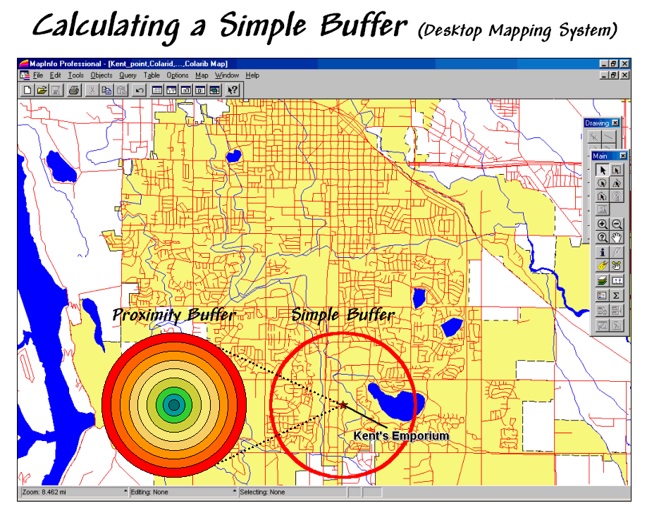
Figure 1. A simple buffer identifies the area within a
specified distance.
Figure 2 outlines a grid-based approach for calculating an effective buffer based on travel-time along the street network. The first step is to export the store and street locations from the desktop mapping system to a grid-based one. Inset (a) depicts the superimposition of a 100-column by 100-row analysis grid over an area of interest. In effect, the data exchange “burns” the store location into its corresponding grid cell (inset b). Similarly, cells containing primary and residential streets are identified (inset c) in a manner analogous to a branding iron burning the street pattern into another grid layer.
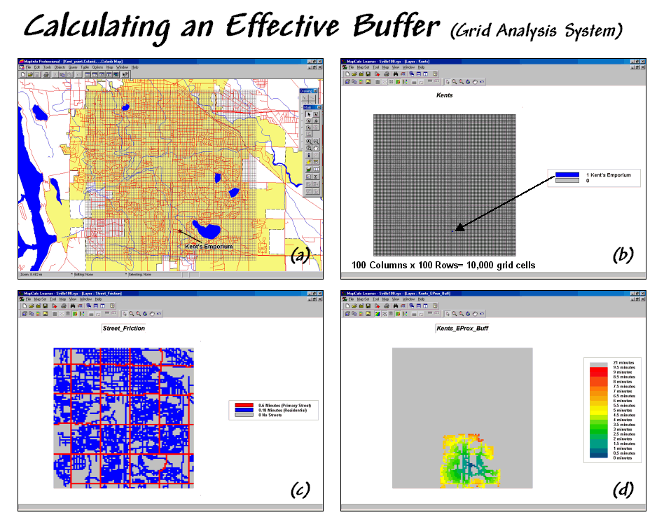
Figure 2. An effective buffer characterizes travel-time
about a map feature.
Inset (d) shows a travel-time buffer derived from the two grid layers. The Store map identifies the starting location and the Streets map identifies the relative ease of travel. Primary streets are the easiest (.1 minute per cell), secondary streets are slower (.3 minute) and non-road areas can’t be crossed at all (infinity). The result is a buffer that looks like a spider’s web with color zones assigned indicating travel-time from 0 to 9.5 minutes away (buffer reach).
While the effective proximity buffer contains more realistic information than the simple buffer, it isn’t perfect. The calibration for the friction surface (inset c) assumed a generalized “average speed” for the street types without consideration of one-way streets, left-turns, school zones and the like. Network analysis packages are designed for such detailed routing. Grid analysis packages, on the other hand, are not designed for navigation but for map analysis. As in most strategic planning it involves a statistical representation of geographic space.
Network and grid-based analysis both struggle with the effects of artificial edges. Some of the streets within the analysis window could be designated as infinitely far away because their connectivity is broken by the window’s border. In addition if the grid cells are large, false connections can be implied by closely aligned yet separate streets.
Generally speaking, the analysis window should extend a bit beyond the specific area of interest and contain cells that are as small as possible. The rub is that large grid maps exponentially affect performance. While the 10,000-cell grid in the example took less than a second to calculate, a 1,000,000-cell grid could take a couple of minutes. The larger maps also require more storage and adversely affect the transfer of information between grid systems and desktop mapping systems. A user must weigh the errors and inaccuracies of a simple buffer against the added requirements of grid processing. However as grid software matures and computers become increasingly more powerful, the decision tips toward the increased use of effective proximity.
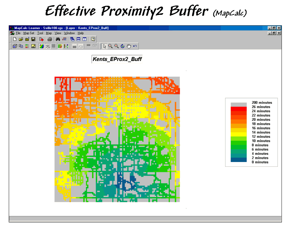
Figure 3. The reach of the travel-time buffer can be
extended to the entire analysis grid.
Figure 3 extends the reach to encompass the entire analysis grid. Note that the farthest location from the store appears to be 26 minutes and is located in the northwest corner. While the proximity pattern has the general shape of concentric circles, the effects of different speeds tend to stretch the results in the directions of the primary streets.
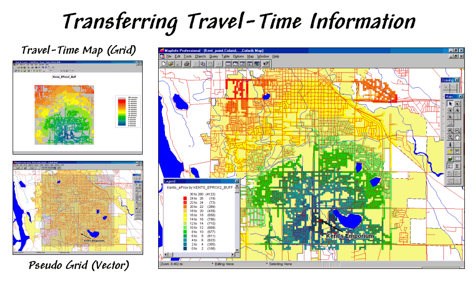
Figure 4. The
travel-time map can be imported into most generic desktop mapping systems by
establishing a pseudo grid.
The information derived in the grid package is easily transferred to a desktop mapping system as standard tables, such as ArcView’s .SHP or MapInfo’s .TAB formats. In a sense, the process simply reverses the “burning” of information used to establish the Store and Street layers (see figure 4). A pseudo grid is generated that represents each cell of the analysis grid as a polygon with the grid information attached as its attributes. The result is polygon map with an interesting spatial pattern—all of the polygons are identical squares that abut one another.
Classifying the pseudo grid polygons into travel-time intervals generated the large display in figure 4. Each polygon is assigned the appropriate color-fill and displayed as a backdrop to the line work of the streets. More importantly, the travel-time values themselves can be merged with any other map layer, such as “appending” the file of the store’s customers with a new field identifying their effective proximity… but that discussion is reserved for next month.
Integrate
Travel-Time into Mapping Packages
(GeoWorld, March 2001, pg. 24-25)
The previous section described a procedure for calculating travel-time buffers and entire grid surfaces. It involves establishing an appropriate analysis grid then transferring the point, line or polygon features that will serve as the starting point (e.g., a store location) and the relative/absolute barriers to travel (e.g., a street map). The analytical operation simulates movement from the starting location to all other map locations and assigns the shortest distance respecting the relative/absolute barriers. If the relative barrier map is calibrated in units of time, the result is a Travel-Time map that depicts the time it takes to travel from the starting point to any map location.
This month’s discussion focuses on how travel-time information can be integrated and utilized in a traditional desktop mapping system. In many applications, base maps are stored in vector-based mapping system then transferred to a grid-based package for analysis of spatial relationships, such as travel-time. The result is transferred back to the mapping system for display and integration with other mapped data, such as customer records.
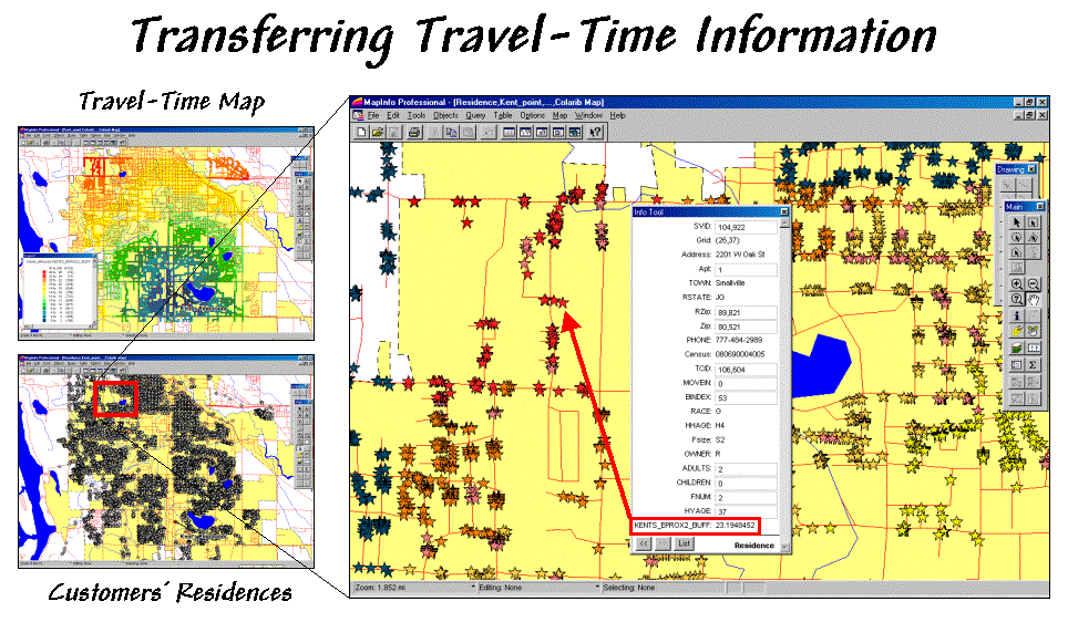
Figure 1. Travel-time and customer information can be
joined to append the effective distance from a store for each customer.
The small map in the top-left of figure 1 is a display of the travel-time map developed last month. The discussion described a procedure for transferring grid-derived information (raster) to desktop mapping systems (vector).
Recall that in a vector system this map is stored as a “pseudo grid” with a separate polygon representing each grid cell—100 columns times 100 rows= 10,000 polygons in this example. While that is a lot of polygons they are simply contiguous squares defined by four lines and are easily stored. The cells serve as a consistent parceling of the study area and any information derived during grid processing is simply transferred and appended as another column to the pseudo grid’s data table.
But how is this
grid information integrated with the data tables defining other maps? For example, one might want to assign a
computed travel-time value to each customer’s record identifying residence
(spatial location) and demographic (descriptive attributes) information. The small map in the bottom-left of figure 1
depicts the residences of the customers of
Most desktop mapping systems provide a feature for “spatially joining” two tables. For example, MapInfo’s “Update Column” tool can be used for the join as specified as “…where object from table <Sville100> contains object from table <Residences>”— Sville100 is the pseudo grid and Residences is the point map (see figure 2). The procedure determines which grid cell contains a customer point then appends the travel-time information for that cell (K_TTime) to the customer record. The process is repeated for all of the customer records and the transferred information becomes a permanent attribute in the Residences table.
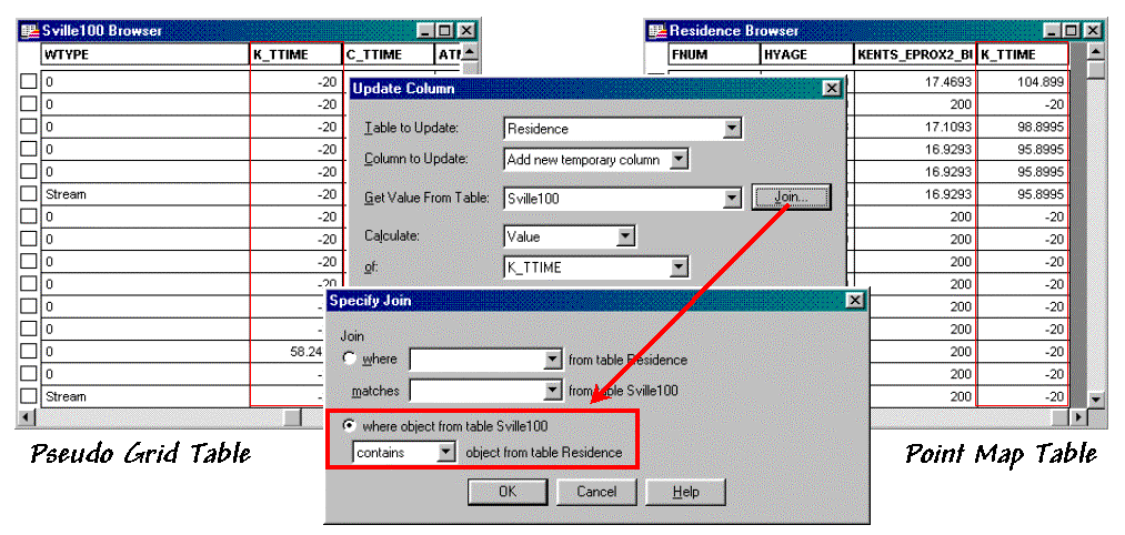
Figure 2. A “spatial join” identifies points that are
contained within each grid cell then appends the information to point records.
The result is shown in the large map on the right side of figure 1. The stars that identify customers’ residences are assigned “colors” depicting their distance from the store. The “info tool” shows the specific distance that was appended to a customer’s record. At this point, the derived travel-time information is fully available in the desktop mapping system for traditional thematic mapping and geo-query processing.
For example, the updated residence table can be searched for customers that are far from the store and have more than three children. The dialog box in the lower right corner of figure 3 shows the specific query statement.
The result is a selection table that contains just the customers who satisfy the query. The map display in figure 3 plots these customers and shows a “hot link” between the selection table and one of the customers with three children who live 10.6 minutes from the store.
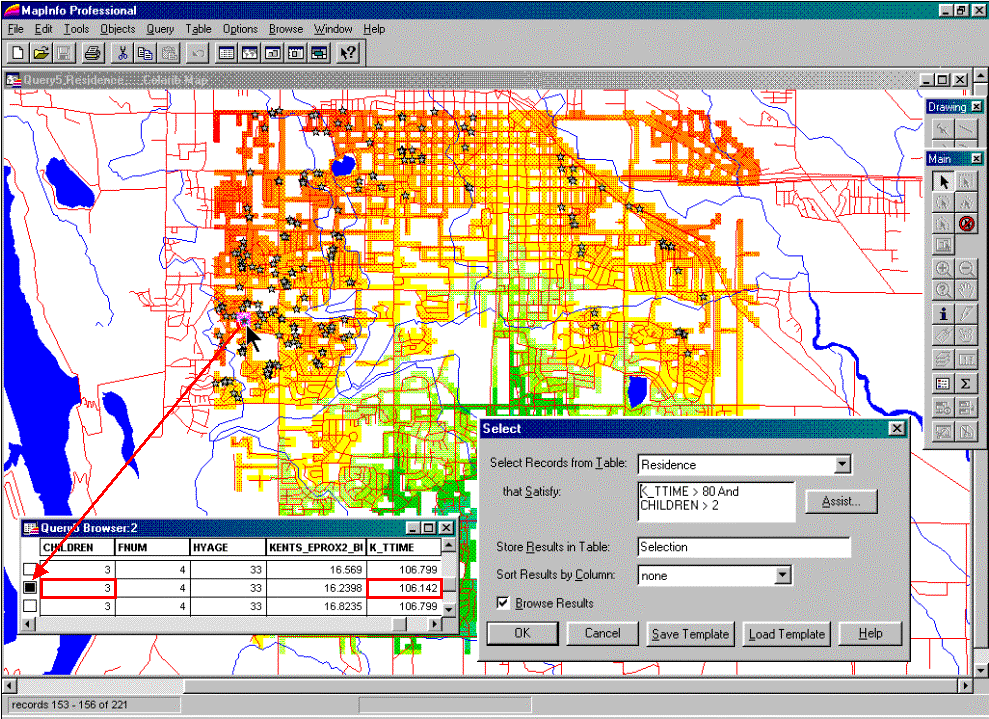
Figure 3. The
appended travel-time information can be utilized in traditional geo-query and
display.
The ability to easily integrate travel-time information greatly enhances traditional descriptive customer information. For example, large families might be a central marketing focus and segmenting these customers by travel-time could provide important insight for retaining customer loyalty. Special mailings and targeted advertising could be made to these distant customers.
Applications that benefit from integrating grid-analysis and
geo-query are numerous. However
traditionally, the processing capability was limited to large and complex
As awareness of grid-analysis capabilities increases and applications crystallize, expect to see more map analysis capabilities and a tighter integration between the raster and vector worlds. In the not so distant future all PC systems will have a travel-time button and wizard that steps you through calculation and integration of the derived mapped data.
Derive and
Use Hiking-Time Maps for Off-Road Travel
(GeoWorld, April 2001, pg. 26-27)
Travel-time maps are most often used within the context of a road system connecting people with places via their cars. Network software is ideal for routing vehicles by optimal paths that account for various types of roads, one-way streets, intersection stoppages and left/right turn delays. The routing information is relatively precise and users can specify preferences for their trip—shortest route, fastest route and even the most scenic route.
In a way, network programs operate similar to the grid-based travel-time procedure discussed in the last two columns. The cells are replaced by line segments, yet the same basic concepts apply—absolute barriers (anywhere off roads) and relative barriers (comparative impedance on roads).
However, there are significant differences in the information produced and how it is used. Network analysis produces exact results necessary for navigation between points. Grid-based travel-time analysis produces statistical results characterizing regions of influence (i.e., effective buffers). Both approaches generate valid and useful information within the context of an application. One shouldn’t use a statistical travel-time map for routing an emergency vehicle. Nor should one use a point-to-point network solution for site location or competition analysis within a decision-making context.
Neither does one apply on-road travel-time analysis when modeling off-road movement. Let’s assume you are a hiker and live at the ranch depicted in figure 1. The top two “floating” map layers on the left identify Roads and Cover_type in the area that affect off-road travel. The Locations map positions the ranch and a nearby cabin.
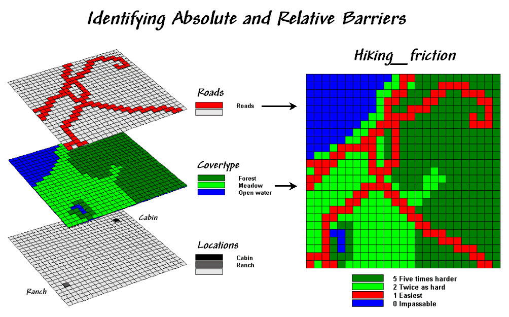
Figure 1. Maps of
Cover Type and Roads are combined and reclassified for relative and absolute
barriers to hiking.
In general, walking along the rural road is easiest and takes about a minute to traverse one of the grid cells. Hiking in the meadow takes twice as long (about two minutes). Hiking in the dense forest, however is much more difficult, and takes about five minutes per cell. Walking on open water presents a real problem for most mortals (absolute barrier) and is assigned zero in the Hiking_friction map on the right that combines the information.
Now the stage is set for calculating foot-traffic throughout the entire project area. Figure 2 shows the result of simulating hiking from the Ranch to everywhere using the “splash” procedure described in the previous two columns. The distance waves move out from the ranch like a “rubber ruler” that bends, expands and contracts as influenced by the barriers on the Hiking_friction map—fast in the easy areas, slow in the harder areas and not at all where there is an absolute barrier.
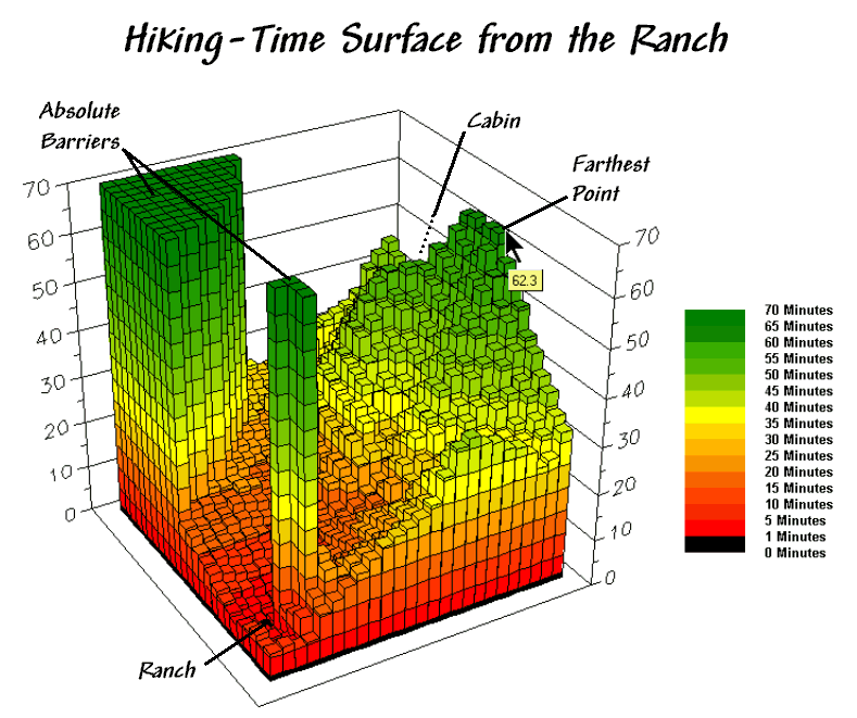
Figure 2. The
hiking-time surface identifies the estimated time to hike from the Ranch to any
other location in the area. The
protruding plateaus identify inaccessible areas (absolute barriers) and are
considered infinitely far away.
The result of the calculations identify a travel-time surface where the map values indicate the hiking time from the Ranch to all other map locations. For example, the estimated time to slog to the farthest point is about 62 minutes. However, the quickest hiking route is not likely a straight line to the ranch, as such a route would require a lot of trail-whacking through the dense forest.
The surface values identify the shortest hiking time to any location. Similarly, the values around a location identify the relative hiking times for adjacent locations. “Optimal” movement from a location toward the ranch chooses the lowest value in the neighborhood—one step closer to the ranch.
The “not-necessarily-straight” route that connects any location to the ranch by the quickest pathway is determined by repeatedly moving to the lowest value along the surface at each step—the steepest downhill path. Like rain running down a hillside, the unique configuration of the surface guides the movement. In this case, however, the guiding surface is a function of the relative ease of hiking under different Roads and Cover_type conditions.
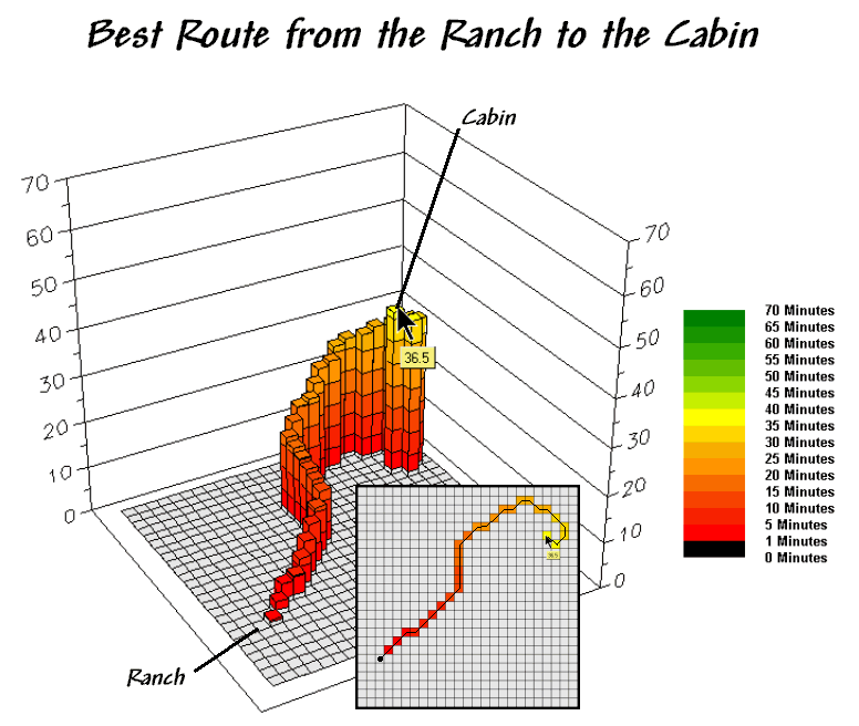
Figure 3. The
steepest downhill path from a location (Cabin) identifies the “best” route
between that location and the starter location (Ranch).
Actually, the optimal path retraces the effective distance wave that got to a location first—the quickest route in this case. The 3D display in figure 3 isolates the optimal path from the ranch to the cabin. The surface value (36.5) identifies that the cabin is about a 36-minute hike from the ranch.
The 2D map depicts the route and can be converted to X,Y
coordinates that serve as waypoints for
________________________
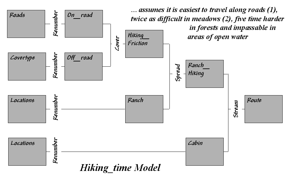
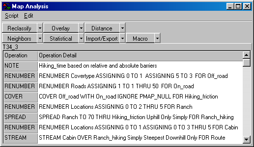
Author’s Note: The following is a flowchart and command macro of
the processing steps described in above discussion. The commands can be entered into the MapCalc
Learner educational software for a hands-on experience in deriving
hiking-time maps.
Consider
Slope and Scenic Beauty in Deriving Hiking Maps
(GeoWorld, May 2001, pg. 24-25)
“It’s the second mouse that gets the cheese.” While effective proximity and travel-time procedures
have been around for years, it is only recently that they are being fully
integrated into
Distance measurement as the “shortest, straight line between two points” has been with us the for thousands of years. The application of the Pythagorean Theorem for measuring distance is both conceptually and mechanically simple. However in the real world, things rarely conform to the simplifying assumptions that all movement is between two points and in a straight line.
Last month’s column described a procedure for calculating a hiking-time map. The approach eliminated the assumption that all measurement is between two points and evolved the concept of distance to one of proximity. The introduction of absolute and relative barriers addressed the other assumption that all movement is in a straight line and extended the concept a bit further to that of effective proximity. The discussion ended with how the hiking-time surface is used to identify an optimal path from any location to the starting location—the shortest but not necessarily straight route.
Now the stage is set to take the concept a few more steps. The top right map in figure 1 is the friction map used last time in deriving the hiking-time surface. It assumes that it takes 1 minute to hike across a road cell, 2 minutes for a meadow cell, and 3 minutes for a forested one. Open water is assigned 0 as you can’t walk on water and it takes zero minutes to be completely submerged. But what about slope? Isn’t it harder to hike on steep slopes regardless of the land cover?
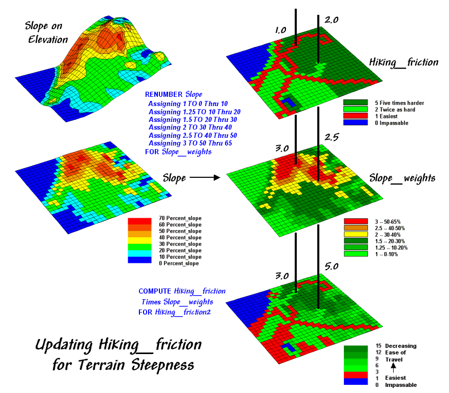
Figure 1. Hiking friction based on Cover Type and Roads
is updated by terrain slope with steeper locations increasing hiking friction.
The slope map on the left side of the figure identifies areas of increasing inclination. The “Renumber” statement assigns a weight (figuratively and literally) to various steepness classes— a factor of 1.0 for gently sloped areas through a factor 3.0 for very steep areas. The “Compute” operation multiplies the map of Hiking_friction times the Slope_weights map. For example, a road location (1 minute) is multiplied by the factor for a steep area (3.0 weight) to increase that location’s friction to 3.0 minutes. Similarly, a meadow location (2 minutes) on a moderately step slope (2.5 weight) results in 5.0 minutes to cross.
The effect of the updated friction map is shown in the top portion of figure 2. Viewing left to right, the first map shows simple friction based solely on land cover features. The second map shows the slope weights calibrated from the slope map. The third one identifies the updated friction map derived by combining the previous two maps.
The 3D surface shows the hiking-time from the ranch to all other locations. The two tall pillars identify areas of open water that are infinitely far away to a hiker. The relative heights along the surface show hiking-time with larger values indicating locations that are farther away. The farthest location (highest hill top) is estimated to be 112 minutes away. That’s nearly twice as long as the estimate using the simple friction map presented last month—those steep slopes really take it out of you.
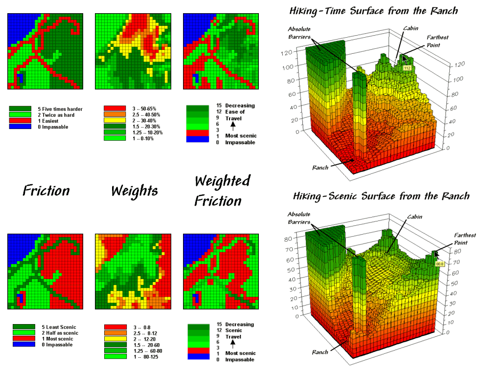
Figure 2. Hiking movement can be based on the time it
takes move throughout a study area, or a less traditional consideration of the
relative scenic beauty encountered through movement.
The lower set of maps in figure 2 reflects an entirely different perspective. In this case, the weights map is based on aesthetics with good views of water enhancing a hiking experience. While the specifics of deriving a “good views of water” map is reserved for next month, it is sufficient to think of it as analogous to a slope map. Areas that are visually connected to the lakes are ideal for hiking. much like areas of gentle terrain. Conversely, areas without such views are less desirable comparable to steep slopes.
The map processing steps for considering aesthetics are identical—calibrate the visual exposure map for a Beauty_weights map and multiply it times the basic Hiking_friction map. The affect is that areas with good views receive smaller friction values and the resulting map surface is biased toward more beautiful hikes. Note the dramatic differences in the two effective proximity surfaces. The top surface is calibrated in comfortable units of minutes. But the bottom one is a bit strange as it implies accumulated scenic beauty while respecting the relative ease of movement in different land cover.
The pair of hiking paths depicted in figure 3 identify significantly different hiking experiences. Both represent an optimal path between the ranch and the cabin, however the red one is the quickest, while the green one is the most beautiful. As discussed last month, an optimal route is identified by the “steepest downhill path” along a proximity surface. In this case the surfaces are radically different (time vs. scenic factors) so the resulting paths are fairly dissimilar.
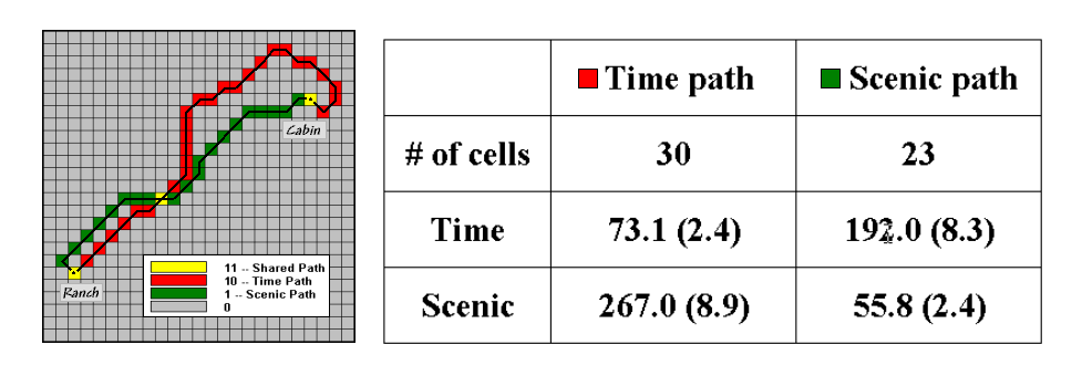
Figure 3. The “best” routes between the Cabin and the
Ranch can be compared by hiking time and scenic beauty.
The table in the figure provides a comparison of the two paths. The number of cells approximates the length of the paths—a lot a longer for the “Time path” route (30 vs. 23 cells). The estimated time entries, however, show that the “Time path” route is much quicker (73 vs. 192 minutes). The scenic entries in the table favor the “Scenic path” (267 vs. 56). The values in parentheses report the averages per cell.
But what about a route that balances time and scenic considerations? A simple approach would average the two weighting maps, then apply the result to the basic friction map. That would assume that time loss in very steep areas is compensated by gains in scenic beauty. Ideally, one would want to bias a hike toward gently sloping areas that have a good view of the lakes.
How about a weighted average where slope or beauty is
treated as more important? What about
hiking considerations other than slope and beauty? What about hiking trail construction and
maintenance concerns? What about
seasonal effects? …that’s the beauty of
____________________________________

Command macro of the processing steps described in
above discussion. The commands can be
entered into the MapCalc
Learner educational software for a hands-on experience in deriving
hiking-time maps.