|
Beyond Mapping II Topic 6: Alternate Data
Structures |
Spatial
Reasoning book |
Are You a GIS Dead-head? — describes
the basics of raster (grid-based) data structure
Raster Is Faster, but Vector Is
Corrector — describes the basics
of vector (line-based) data structure
How’s Your Quads and TINs? — describes
commonly used alternative raster and vector data structures
Rasterized Lines and Vectorized
Cells — describes uncommonly alternative raster and
vector data structures
<Click here> for
a printer-friendly version of this topic (.pdf).
(Back to the Table of Contents)
______________________________
Are You a GIS Dead-head?
(GeoWorld,
)
Even
if you are new to GIS you must have encountered the scholarly skirmishes
between the raster-heads and the vector-heads.
Like other religious crusades the principles in these debates are
frequently lost to mindsets reflecting cultural exposure and past
experience. However, more often than
not, most of us just become catatonic when the discussion turns to GIS data
structures. But what the heck, it's
worth another try.
Let's
review the basic tenets of vector and raster data (Beyond Mapping columns July
through September, 1993) then extend this knowledge to the actual data
structures involved. Vector data uses
sets of X, Y coordinates
to locate three basic types of landscape features— points, lines and
areas. For example, a typical water map
identifies a spring as a dot (one X,Y coordinate pair), a stream as a squiggle
(a set of connected X,Y coordinates) and a lake as a glob (a set of connected
X,Y coordinates closing on itself and implying its interior). Raster, on the other hand, uses an imaginary
grid of cells to represent the landscape.
Point features are stored as individual Column, Row entries in the grid; lines are identified as a set
of connected cells; and areas are distinguished as all of the cells comprising
a feature.
This
traditional representation constrains geographical phenomenon to three
user-defined conditions (points, lines and areas) and two GIS expressions
(vector and raster). I bet this
conceptual organization is fairly comfortable, and might even be familiar. But that's only half the problem— this user/GIS
representation has to be translated into a database/hardware structure.
At this step most of us simply glaze-over and leave such details to the
GIS jocks. Actually, the concepts aren't
all that hard and they can explain a lot about different systems, frustrations
you encounter and future directions of GIS.
Let's
consider some structures for raster data.
The left side of figure 1 shows an imaginary grid superimposed on a
typical soil map (more appropriately termed a "data layer"). The center portion of the figure identifies a
matrix of numbers with a
numerical value assigned to each cell.
In this case, the value represents a particular type of soil and it's
positioning in the matrix indicates its location. To the computer, however, the matrix isn't a
2-dimensional array; it’s simply one long list of numbers. The first number represents the upper-left
corner of the matrix, and rest are ordered like you would read a book— from
left to right, top to bottom. Another
map for the same area, say elevation, would be stored as a separate ordered sequential file. This is the simplest and most frequently used
raster data structure.
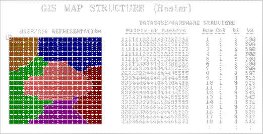
Figure
1. Raster
Data Structure Elements. A file containing
a matrix of numbers (attribute values) characterizes each cell of an imaginary
grid. An alternative structure uses a
standard database file containing the column/row identifiers for each cell
followed by attribute fields, such as soil type and elevation.
An
offshoot of this structure is used for most remote sensing data. Each cell in the grid represents a small area
on the earth's surface where the satellite collected "spectral
data." The numbers it collects
record the relative amounts of energy, such as blue, green and red light
radiating from the surface. The set of
values for each energy level represents a single data layer which could be
arranged as a matrix and stored separately as noted above. These data, however, are more efficiently
stored as an interlaced matrix
with all of the measurements for each cell sequentially stored. For example, the first three values might
represent the blue, green and red light measurements for the upper-left cell
with the following triplets of values for the other cells sequenced left to
right, top to bottom as before.
The
interlaced structure has a significant advantage in point-by-point processing because
all information is contained in a single file and readily available as the
computer methodically steps through the matrix.
It doesn't have to open three separate files, and then read blue, green
and red values that scattered all over the disk. That means a lot less disk-thrashing and a
whole lot happier computer. This might
not seem a big deal to you, but considering that a typical Landsat TM scene
contains seven data layers for about 36 million cells (that's over 250 million
numbers!), even a slight increase in storage efficiency is cyber heaven.
The
interlaced structure might be neat and tidy for remote sensing data, but it is
inappropriate for a general GIS. First,
it's tough to add a new map. It means
that extra room must be made to insert the new values by reading the first
three values from the original file, writing them to a new file, inserting the
first new value, then repeat the process for the other million or so cells...
oh yes, then delete the original file.
And you have the same problem if you want to delete a map. Secondly, since the information for each data
layer is dispersed (every third value), it is difficult to compress the
redundancy found in a typical map.
Finally, any processing involving neighboring cells requires extra work
as the computer must continually jump back and forth in the file to get values
for the cells above, below, right and left of the target cell. In short, the interlaced structure is best
for specialized applications involving a fixed number of maps constrained to
point-by-point processing.
So
what else do we have in raster structures?
Consider the right side of the figure.
This structure uses a standard database file (termed a "database
table") with the column, row entries of the matrix explicitly stored as
"fields" (i.e., separate columns).
The subsequent fields contain the listing of values for various data
layers. Note that the set of soil values
under the V1 heading correspond to the left-most column of the matrix. If there was room in the figure to list the
rest of the values in the field, the next set would replicate the next column
to the right in the matrix, then the next, and so on. The V2 listing depicts elevation values,
similarly organized.
Now
comes the advantage... suppose you wanted to find all locations (i.e., cells)
which contain soil type 4 and are over 550 feet in elevation. Simply enter an SQL (sequential query
language) command and the computer searches V1 and V2 for the specified condition. A new field (V3) will be appended containing
the results. It is a piece-of-cake
because you are using a standard database file under the control of a standard
database management program. This
standardized structure makes it easy for the GIS programmer as he doesn't have
to write all the code that is already in the database "engine." Also, it allows you to store and process text
string designations, as well as numerical values. More importantly, it makes it easy on the
user as the command uses the same format as a normal office database.
The
problem is with the computer. It hates
appending new fields to an existing table.
Also, the number of fields in a single table is severely constrained. The solution is a series of indexed tables with each cell's
designation serving as the common link.
With an indexed structure the computer can easily "thread"
from one table to another. Actually,
there are good arguments to store each data layer as a separate indexed
table. Creation, modification and
deletion of a map is a breeze as it affects only one table, rather than an
embedded field in a complex table. That
seems to bring us back to where we began— one map, one file. But in this instance, each map is a standard
indexed database table with all of the rights, privileges and responsibilities
of your office database. It puts raster
GIS where it should be... right in the midst of standard database
technology. As we will se next month,
vector GIS has been there all along.
Raster Is Faster, but
Vector Is Corrector
(GeoWorld,
)
Your
computer really loves raster data— a cell on one map is at the same position as
on all others. A couple of
"hits-to-disk" and it knows everything about a cell location. A few more hits up, down, left and right and
it knows everything about a location's entire neighborhood. If fact, it can "walk" from one
location to another and find everything it needs to know along the way, right
from the hard disk. Its world is
pre-defined in little byte size pieces that are just right.
However,
it's the computer-endearing qualities of consistency and uniformity that makes
raster data at odds with the human psychy (and a lot of reality). We see the unique character of each map
feature— a cute little jog here, a little bulge over there. The thought of generalizing these details
into a set of uniform globbies is cartographic heresy.
So
what does it cost your computer, in terms of data structure, to retain the
spatial precision you demand? First,
because every map feature is unique, a more complicated data structure is
required. Consistency and uniformity are
out; uniqueness and irregularity are in.
More importantly, processing involves threading through a series of
linked files (termed tables in DB-speak), mathematically constructing map
features, calculating the implied coincidence, then reconstructing the new data
structure linkages. All this just to
know that the property line isn't a hundred feet over there... picky, picky.
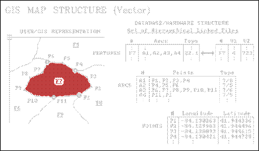
Figure 1. Vector Data Structure Elements. A set of files links coordinates, arcs and
features to describe location. A
standard database file links each feature to its attributes, such as soil type
and elevation.
Figure
1 identifies the basic elements of vector data structure. It begins with a points table attaching coordinates to each point used in the
construction of map features. Most
systems use latitude and longitude as their base coordinates. This is a good choice as it is a spherical
coordinate system accurately locating points anywhere on the Earth's
surface. However, it is a problem
whenever you want to relate points, such as measuring distances, bearings or
areas. In three dimensions seemingly
simple calculations involve solid geometry and ugly equations that bring even
powerful computers into their knees.
Plus, the 3-dimensional answers can't be drawn on a flat screen. The solution is to carry a user-specified map
projection scheme and planar coordinate system (e.g., Universal Transverse
Mercator), then translate on-the-fly.
Now the computer can work in any 2-dimensional rendering you choose and
easily display the results on your screen or plotter... happy computer, happy
you.
For
point features, the point table and its 2-D translation specifications are
directly linked to another indexed file containing descriptive information,
termed attributes, about each point. If
this information depicted soil samples, you could query the attribute table for
all of the samples that have a PH less than 7 and available phosphorous
exceeding 30 parts per million. The
results from the attribute query simply "threads" to the coordinates
of the subset of points meeting the conditions, then plots them at blinding
speed in the vibrant color of your choice.
Line
and area features are a bit more complicated because the various connections
among sets of points need to be specified.
When you view a human-compatible map of water features you intuitively note
which stream is connected to which stream by the network of blue
squiggles. You note lakes are blue globs
with a squiggle in and another out. But
the computer's point file is just a huge pile of unrelated numbers. The first level of organization is a linked arcs table. This file groups the points into connected
sets of arcs forming the map features.
In the figure points P1, P2, P3 and P4 are connected to form arc A1. Arcs A2, A3, and A4 are similarly defined by
their linked coordinates.
The
features table puts it
all together in geographic space by linking the arcs to actual map
features. In the example, feature F7 is
formed by linking arcs A1, A2, A3, and A4.
The corresponding arcs table identifies which points are involved, with
the coordinates in the points table ultimately tying everything to the
ground. At the top of this scheme is a
linked info table with
the attribute data for each map feature.
In the example, feature F7 is identified as having soil type 4 (V1) and
an average elevation of 723 (V2).
There,
that's not too bad— conceptually. The
tough part comes when you try to put it all into practice with about 100,000
polygons. That's where each vendor's
"secrete ingredients" to the general vector recipe take hold. Without giving away any corporate secretes,
let's take a look at some of the "tweaking" possibilities.
In
addition to the link to the points, the arcs and feature tables often contains “topological”
(geometric relationships among the points, lines and polygons) and other
sundry information. For example, note
that arc A1 forms a shared boundary between features F7 and F8 as listed in the
"Topo" field of the arcs table (7/8).
For maps composed of contiguous polygons (e.g., soils, covertype,
ownership, and census tracks) a search of this field immediately identifies the
adjoining neighbors for any map feature.
Many systems store frequently used geometric measurements, such area as
depicted in the "Topo" field of the features table (22.1 acres). The alternative to these tweaks in data
structure design is a lot of computational thrashing and bashing each time they
are needed.
Line
networks use topological information to establish which arcs are interconnected
and the nature of their connections. In
a stream network it depicts the direction of water flow. In a road network, it characterizes all
possible routes from any location to all other locations. However, to fully describe this linkage a new
element must be introduced— the node. These special points are indicated in the
figure as the large dots at the ends of each arc (P1, P4, P6, and P11). Nodes represent locations where things are
changing, such as the separation of adjacent soil units along a soil
boundary. Some systems store nodes in a
separate table, while others simply give them special recognition in the points
table. The information associated with a
node is a reflection of the type of data and the intended processing.
If
the length of each arc is stored, the computer can find the distance from a
location to all other locations by simply summing the intervening arcs along a
route. If an average speed is stored for
each arc, the answer will be in travel-time.
But what about one-way streets and the relative difficulty of left and
right turns at each intersection (i.e., node)?
Attach this information to the nodes and the computer will make the
appropriate corrections as it encounters the intersections along a route. Similarly, an accumulated distance from a
location to its surroundings can be determined by keeping a running sum of the
arc distances, respecting the "turntable" information at each
node. Once this is known it is an easy
matter to determine the "optimal path" (shortest time or distance)
from any location to the starting point.
But
all is for not if your data structure hasn't been "tweaked" to carry
the extra topological and calibration information. It should be apparent that, unlike raster,
vector data structures can be radically different. Ingenuity and programming dexterity are
critical factors, as is the matching of data design to intended applications
and hardware. That's the tough part...
there isn't a "universal truth" in vector data structure. The onus is on you to pick the right one for
your applications, and then understand it enough to take it to its limits.
(GeoWorld,
)
Original
flavored raster and vector data structures have been around for a long
time. The basic concepts in representing
a landscape as a set of grid cells or a set of connected points are about as
old as cartography itself. The technical
refinements required for a functioning GIS, however, are continually
evolving. It seems about the time you
think we have reached the pinnacle of data structure design, someone comes out
with a new offshoot. The only folks that
think they have it all are over-zealous marketers. The technical types keep their heads down,
constantly looking for more effective ways of characterizing mapped data.
Most
raster systems have the ability to perform Run-length Compression that compacts along the rows or the
columns. For example, consider the
following matrix and its row-compressed translation.
Full
Matrix Run-Length
(Row)
111111122222222223 1,7,2,17,3,18
111111122222222233 1,7,2,16,3,18
111111122222222333 1,7,2,15,3,18
111111222222223333 1,6,2,14,3,18
111113333333333333 1,5,3,18
111113333333333333 1,5,3,18
111113333333333333 1,5,3,18
111333333333333333 1,3,3,18
111333333333333333 1,3,3,18
The
run-length data structure uses just 44 numbers to represent the 162 numbers in
the full matrix. It uses "value,
through column" pairs of numbers to compact the redundancy along a
row. For example, the first row is read
"value from column 1 (assumed) through column 7; value 2 from column 8
(last column plus one) through column 17; and value 3 from column 18 through
column 18." This format is
particularly useful in map display.
Instead of "hitting disk" for the color fill pattern value at
each cell, the computer reads the pattern designation and then simply repeats
the pattern as specified by the column spread.
That's both a savings in storage and increased performance— a win, win
situation.
So
why don't we compress in both the row and column directions at the same time
and get even more? In effect, that is
what a Quadtree data structure
does. It is an interesting second cousin
to the traditional raster data structure that uses a cascading set of grid
resolutions to compress redundancy.
Consider the map boundaries shown in Figure 1. If the map window is divided in half in both
the X and Y directions, four panels (quadrants) are identified. This has the effect of superimposing a very
course grid of just two columns and two rows.
At
this point the computer tests if any quadrant wholly contains a single map
characteristic. In the example there are
none, so each panel is divided into their quads (Level 2). At this point, there are seven of the sixteen
quadrants wholly containing a single characteristic. Their positions in the 4x4 grid are noted,
and the remaining nine mixed panels are divided into their quads (Level
3). Fourteen of these are noted as
completed, and the remaining 22 are divided for Level 4 of the quadtree. The process is repeated until an appropriate
quad level resolution is reached. At
level 16, a gridding resolution of 65,536 by 65,536 is available wherever it is
needed... that equates to a fixed raster grid of 4,294,967,296 cells! But the quadtree is not forced to use this
resolution everywhere, and accurately stores most maps in less than a megabyte.
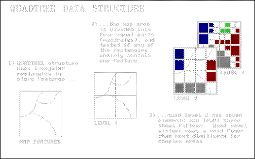
Figure
1. Quadtree
Data Structure Elements.
Quadtrees
and run-length structures are good at compressing raster data. However, they must be decompressed then
recompressed for most map analysis operations.
A lot of GIS systems have chosen not to impose a compression routine
within the data structure, but simply to leave it up to commercial hard disk
compression packages, such as PKWare or Stacker. These packages not only respond to data
redundancy, but optimize for disk head movement as well.
Triangulated
Irregular Network, or TIN data
structure, is a vector offshoot originally designed for elevation
data. It avoids the redundancy of
elevations in a normal raster representation, and is more efficient for some
terrain analysis operations, such as slope and aspect. It uses a set of irregularly spaced elevation
measurements, with intensive sampling in areas of complex relief and/or
important features, such as ridges and streams.
A bit of computer wizardry is applied to determine the network of
triangular facets that best fits these data.
Each facet has three interconnected elevations and can be visualized as
a tilted triangular plane. The direction
cosines of the plane identify its slope and aspect. The average of the three elevations
generalizes the plane's height.
As
shown in Figure 2, the XY coordinate (location) and the Z coordinate
(elevation) are stored in a points table.
Similar to traditional vector structuring, the triangular facets are
defined in a features table by their three nodes and adjoining facets. The final link is to an attribute table
containing descriptive information on each facet. Awesome shaded relief maps can be generated
by plotting the facets in 3-D and shading them as a function of their slope and
aspect.
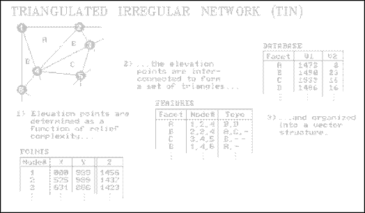
Figure
2. TIN Data
Structure Elements.
Using
a TIN structure, instead of raster, to characterize a 3-D surface has some
significant advantages— it usually requires fewer points, captures
discontinuities like streams and ridges, and determines slope and aspect of the
facet itself. It is the data structure
of choice for most civil engineering packages dominated by terrain
analysis. However, it's inappropriate
for a generalized GIS mixing a variety of maps.
First, it is like raster as it uses a mosaic of geographic chunks to
represent a map feature. However, the
chunks are inconsistent between maps, and something as simple as map overlay
takes a severe hit in performance. Also,
the 2-D renderings of TIN is extremely complex and bewildering to most users
compared to a normal vector plot.
Quadtree
and TIN are useful offshoots of basic raster and vector data structures. They provide important benefits for certain
data under certain conditions... if they match your needs; they're an
invaluable addition to your GIS arsenal.
Rasterized Lines and
Vectorized Cells
(GeoWorld,
)
Rasterized
Lines and Vectorized Cells
Chances
are your GIS is (or will be) ambidextrous.
It will have a vector side and a raster side, and might even have TIN or
quadtree sides. The different data
structures indicate differing perspectives on both data type and user
application. The vector approach
characterizes discrete map objects and was strongly influenced by applications
in computer graphics. Raster, on the
other hand, characterizes continuous mapped data and emerged from remote
sensing applications involving multivariate statistics. Today, considerations
in database/ hardware structure are influencing future development as much as
historical user/GIS representation theory.
In a sense, the realities of an evolving computer environment are
challenging traditional ways.
Rasterized lines are an
interesting offshoot from the traditional data structures. It's sort of a hybrid, as it uses a grid
structure to characterize a map's line-work.
An optical scanner is used to "turn-on" each cell in a fine
sampling matrix that corresponds to the set of lines. This process is similar to your office fax
machine reading a document. The fax at
the other end simply deciphers the on and off conditions in the matrix and
shoots a dab of black ink at spots corresponding to "on." It skips over the "off" spots
leaving just white paper. That's it, a black
and white rendering of the map's lines pushed over the phone lines.
If
you use a magnifying glass, you can actually see the individual dots. But at normal viewing distances they merge to
form smooth lines. Your brain easily
makes sense of the pattern of lines and implied polygons embedded in the fine
grid of the sampling matrix. Which
streams are connected to which streams …and which lakes are in which watersheds
…are obvious from the graphic rendering.
But
that's not the case for a computer... it's just a jumble of on and off
dots. The first step in imposing data
structure order is to locate and mark as nodes the entire set of special dots
where lines meet (intersections), or are just hanging out there by themselves
(end points). Traditional vector
structuring "follows" the dots between nodes, storing the coordinates
for a point whenever there is a significant X or Y deflection. The result is a series of discrete points
connected by implied straight lines, as shown in inset 2 of Figure 1. The nodes and intervening points are then
arranged as series of indexed files, as described in the previous article.
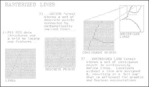
Figure
1.
Rasterized Lines Data Structure Elements.
Rasterized
lines, on the other hand, retain all of the dots along the lines. At first this seems stupid as the points file
is huge. Where an arc might require ten discrete
points, a rasterized line might require a hundred or more. Some tricks in data compression and
coordinate referencing can help, but anyway you look at it storage is a lot
more. So why would anybody use a
rasterized line structure? Primarily because
it is a format hardware loves. Faxes,
scanners, screens, plotters and printers are all based on dot patterns. As a result, there is a lot of attention
being paid to the efficient handling of dotted data. Also, advances in optical disk storage and memory
chips are redefining our concepts of a "storage hog," and these files
seem smaller each year.
More
importantly, however, are the advancements in CPUs (central processing
units). Most computers still use a
"kur-plunk-a" processing approach developed in the 1940's. It mimics our linear thinking and the way we
do things... do A, then B, then C. Array
and parallel processors, on the other hand, simultaneously operate on whole
sets of data, provided they are properly organized.
Suppose
you want to overlay a couple of traditional vector maps. At an instant in time, the computer reads the
coordinates for two points on one map, then has to figure out if the implied
line segment between them crosses any other implied line segment on the other
map. If it does, mathematically
calculate the point of intersection, split the two lines into four, then update
all of the indexed tables... whew! This
approach is not only a lot of work; it's a purely linear process and a miss-match
for array processing.
Figure
2.
Vectorized Cells Data Structure Elements.
If
the data is in rasterized line format, however, an array processor merely reads
the corresponding chunks of cells on both maps, and multiplies them together (a
Boolean operation for you techy types).
The product array identifies the composite of the two maps and
highlights the new nodes where lines crossed.
Don't get me wrong, I am not advocating you run out and buy a rasterized
line system, but it has some interesting features that may play to tomorrow's
computers.
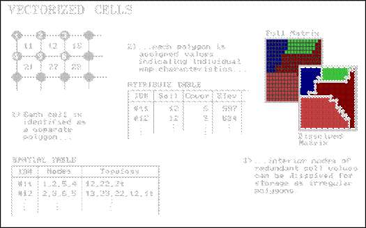
Another
interesting offshoot is Vectorized
cells, as shown in Figure 2.
It cheats by storing each cell of an analysis grid as an individual
polygon. It just happens that all of the
polygons have the same square configuration and adjoin their neighbors. From a traditional vector perspective, each
point defining a cell is a node; each cell side is an arc composed of just two
nodes; and each cell is a polygonal feature composed of just four arcs. This approach utilizes the existing vector
structure without impacting the existing code.
It simply imposes consistency and uniformity in the polygons. All that is needed is an import module to
generate the appropriate configuration of vectorized cells and read the raster
values into a field in the corresponding attribute table. Raster to vector conversion can be completed
by dissolving the "pseudo-boundaries" between adjoining polygons
having the same value. Line features can
be converted by connecting the centers of cells of similar value. Point features are represented by the
coordinates of isolated cell centers.
Vectorized
cells were initially used to "kludge" a link from raster to vector
systems. However, the inherent
consistency and uniformity of the structure (four points to a polygon), coupled
with advances in data compression and database technology might lead to a
resurgence in interest. Things are fluid
as computers are becoming less bounded by storage and the industry is shifting
toward new processors and operating systems.
During all this, keep in mind that there are only two things certain
about data structures— 1) tomorrow there will be another one, and 2) what is
good for one application isn't necessarily the best for another.
______________________________