3D GIS Concepts and Considerations

The excerpts below on 3D GIS Concepts and Considerations are from the Beyond Mapping column in GeoWorld. Online versions of all of the columns in the series from 1996 to the present are available in the online book Beyond Mapping III at www.innovativegis.com/basis/MapAnalysis/ organized as a Chronological Listing or by Topic.

Innovation Drives GIS Evolution, Topic 27— discusses the cyclic nature of GIS innovation (Mapping, Structure and Analysis)

Referencing the Future, Introduction— describes current and alternative approaches for referencing geographic and abstract space

Visualizing a Three-dimensional Reality, Topic 27— uses visual connectivity to introduce and reinforce concepts of 3D geography

Thinking Outside the Box, Topic 27— discusses concepts and configuration of 3-dimensional geography

From a Map Pancake to Soufflé, Topic 27— continues the discussion of concepts and configuration of a 3D GIS

<click here> for a printer-friendly version (.pdf); electronic version at www.innovativegis.com/basis/Papers/Other/3D_GIS/

________________________________________

Innovation Drives GIS Evolution

(GeoWorld August, 2007)

What I find interesting is that current geospatial innovation is being driven more and more by users. In the early years of GIS one would dream up a new spatial widget, code it, and then attempt to explain to others how and why they ought to use it. This sounds a bit like the proverbial “cart in front of the horse” but such backward practical logic is often what moves technology in entirely new directions.

“User-driven innovation,” on the other hand, is in part an oxymoron, as innovation—“a creation, a new device or process resulting from study and experimentation” (Dictionary.com)—is usually thought of as canonic advancements leading technology and not market-driven solutions following demand. At the moment, the over 500 billion dollar advertising market with a rapidly growing share in digital media is dominating attention and the competition for eyeballs is directing geospatial innovation with a host of new display/visualization capabilities.

User-driven GIS innovation will become more and more schizophrenic with a growing gap between the two clans of the GIS user community as shown in figure 1.

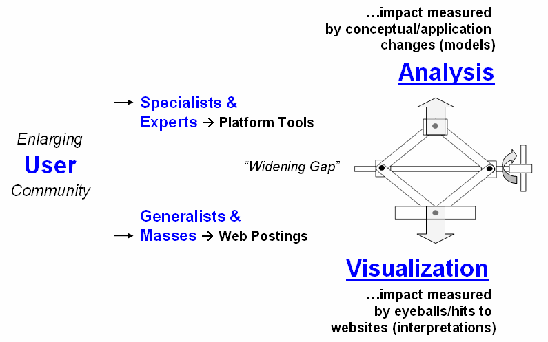
Figure 1. Widening gap in the GIS user community.

Another interesting point is that “radical” innovation often comes from fields with minimal or no paper map legacy, such as agriculture and retail sales, because these fields do not have pre-conceived mapping applications to constrain spatial reasoning and innovation.

In the case of Precision Agriculture, geospatial technology (GIS/RS/GPS) is coupled with robotics for “on-the-fly” data collection and prescription application as tractors move throughout a field. In Geo-business, when you swipe your credit card an analytic process knows what you bought, where you bought it, where you live and can combine this information with lifestyle and demographic data through spatial data mining to derive maps of “propensity to buy” various products throughout a market area. Keep in mind that these map analysis applications were non-existent a dozen years ago but now millions of acres and billions of transactions are part of the geospatial “stone soup” mix.

As shown in figure 2 the evolution of GIS is more cyclical than linear. My greybeard perspective of over 30 years in GIS suggests that we have been here before. In the 1970s the research and early applications centered on Computer Mapping (display focus) that yielded to Spatial Data Management (data structure/management focus) in the next decade as we linked digital maps to attribute databases for geo-query. The 1990s centered on GIS Modeling (analysis focus) that laid the groundwork for whole new ways of assessing spatial patterns and relations, as well as entirely new applications such as precision agriculture and geo-business.

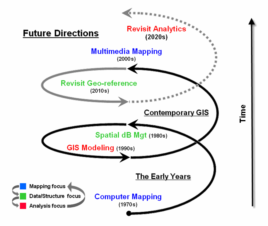
Figure 2. GIS Innovation/Development cycles.

Today, GIS is centered on Multimedia Mapping (mapping focus) which brings us full circle to our beginnings. While advances in virtual reality and 3D visualization can “knock-your-socks-off” they represent incremental progress in visualizing maps that exploit dramatic computer hardware/software advances. The truly geospatial innovation awaits the next re-focusing on data/structure and analysis.

The bulk of the current state of geospatial analysis relies on “static coincidence modeling” using a stack of geo-registered map layers. But the frontier of GIS research is shifting focus to “dynamic flows modeling” that tracks movement over space and time in three-dimensional geographic space. But a wholesale revamping of data structure is needed to make this leap.

The impact of the next decade’s evolution will be huge and shake the very core of GIS—the Cartesian coordinate system itself …a spatial referencing concept introduced by mathematician Rene Descartes 400 years ago.

The current 2D square for geographic referencing is fine for “static coincidence” analysis over relatively small land areas, but woefully lacking for “dynamic 3D flows.” It is likely that Descartes’ 2D squares will be replaced by hexagons (like the patches forming a soccer ball) that better represent our curved earth’s surface …and the 3D cubes replaced by nesting polyhedrals for a consistent and seamless representation of three-dimensional geographic space. This change in referencing extends the current six-sides of a cube for flow modeling to the twelve-sides (facets) of a polyhedral—radically changing our algorithms as well as our historical perspective of mapping (see April 2007 Beyond Mapping column for more discussion).

The new geo-referencing framework provides a needed foothold for solving complex spatial problems, such as intercepting a nuclear missile using supersonic evasive maneuvers or tracking the air, surface and groundwater flows and concentrations of a toxic release. While the advanced map analysis applications coming our way aren’t the bread and butter of mass applications based on historical map usage (visualization and geo-query of data layers) they represent natural extensions of geospatial conceptualization and analysis …built upon an entirely new set analytic tools, geo-referencing framework and a more realistic paradigm of geographic space.

____________________________

Author’s Note: I have been involved in research, teaching, consulting and GIS software development since 1971 and presented my first graduate course in GIS Modeling in 1977. The discussion in these columns is a distillation of this experience and several keynotes, plenary presentations and other papers—many are posted online at www.innovativegis.com/basis/basis/cv_berry.htm.

Referencing the Future

(GeoWorld, April 2007)

Geo-referencing is the cornerstone of GIS. In the mid-1600s the French mathematician, René Descartes established the Cartesian coordinate system that is still in use today. The system determines the location of each point in a plane as defined by two numbers—its x-coordinate and y-coordinate. A third z-coordinate is used to extend the system to 3-dimensional geographic space. In mapping, these coordinates reference a refined ellipsoid (geodetic datum) that can be conceptualized as a curved surface approximating the mean ocean surface of the earth.

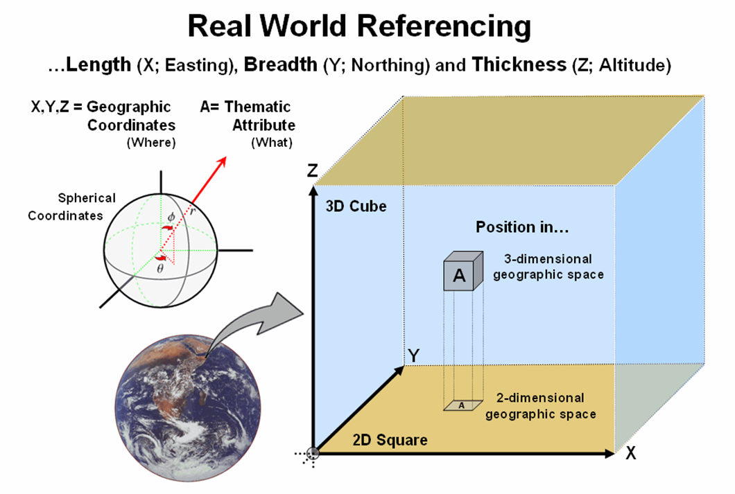
Figure 1. Geographic referencing uses three coordinates to locate map features in real world space.

The location and shape of map features can be established by X and Y distances measured along flattened portions of the reference surface (figure 1). The familiar Universal Transverse Mercator (UTM) coordinates represent E-W and N-S movements in meters along the plane. The rub is that UTM zones are need to break the curved earth surface into a series of small flat, projected subsections that are difficult to edge-match.

A variant of the traditional referencing system uses spherical coordinates that are based on solid angles measured from the center of the earth. This natural form for describing positions on a sphere is defined by three coordinates—an azimuthal angle (θ) in the X,Y plane from the x-axis, the polar angle (φ) from the z-axis, and the radial distance (r) from the earth’s center (origin). The advantage of a spherical referencing system is that it is seamless throughout the globe and doesn’t require projecting to a localized flat plane.

Digital map storage is rapidly moving toward spherical referencing that uses latitude and longitude in decimal degrees for internal storage and on-the-fly conversion to any planar projection. This radical change from our paper map heritage is fueled by ubiquitous use of GPS and a desire for global databases that easily walk across political and administrative boundaries.

Since the digital map is a radical departure from the paper map, other alternative referencing schemes are possible. For example, hexagons can replace the Cartesian grid squares we have used for hundreds of years (top portion of figure 2). The hexagon naturally nests to form a continuous network like a beehive’s honeycomb. An important property of a hexagon grid is that it better represents curved surfaces than a square grid— a socccer ball stiched from squares wouldn’t roll the same.

However the most important property is that a hexagon has six sides instead of four. The added directions provide a foothold for more precise measurement of continuous movement— one can turn right- and left-oblique as well as just right and left. Traditional routing models using Least Cost Path would benefit greatly.

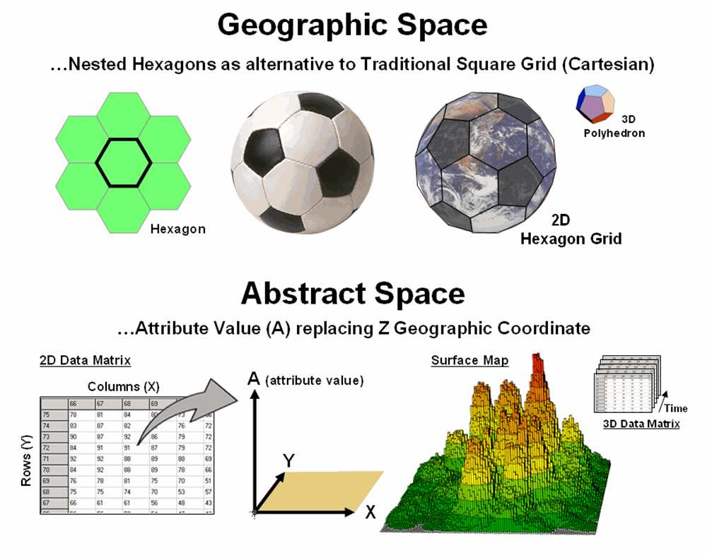
Figure 2. Alternative referencing systems and abstract space characterization are possible through the digital nature of modern maps.

Expanding to 3-dimensional geographic space provides for polyhedrons to replace cubes. For example, a dodecahedron is a nesting twelve-sided object that can be used instead of the six-sided cube. Weather and ground water flow modeling could be greatly enhanced by the increased options for transfer from a location to its larger set of adjoining locations. The computations for cross-products of vectors, such as warp-speed cruise missiles, could be greatly assisted as they are affected by different atmospheric conditions and evasive trajectories.

Another extension involves the use of abstract space (bottom portion of figure 2). For example, the Z-coordinate can be replaced with an attribute value to generate a map surface, such as customer density. In this instance, the abstract referencing is a mixture of spatial and attribute “coordinates” and doesn’t imply 3-dimensional, real word geographic occurrences. Instead, it relates geography and conditions in an extremely useful way for conceptualizing patterns. Normalization along the abstract coordinate axis is an important consideration for both visualization and analysis.

This brings us to space-time referencing. During a recent panel discussion I was challenged for suggesting such a combination is possible within a GIS. The idea has been debated for years by philosophers and physicists but H.G. Wells’ succinct description is one of the best—

'Clearly,' the Time Traveller proceeded, 'any real body must have extension in four directions: it must have Length, Breadth, Thickness, and - Duration. But through a natural infirmity of the flesh, which I will explain to you in a moment, we incline to overlook this fact. There are really four dimensions, three which we call the three planes of Space, and a fourth, Time. There is, however, a tendency to draw an unreal distinction between the former three dimensions and the latter, because it happens that our consciousness moves intermittently in one direction along the latter from the beginning to the end of our lives.' (Chapter 1, Time Machine).

The upshot seems to be that a fourth dimension exists (see Author’s Notes), it is just you can’t go there in person. But a GIS can easily take you there - conceptually. For example, an additional abstract “coordinate” representing time can be added to form a 3-dimentional data matrix. The GIS picks off the customer density data for the first “page” and displays it as in the figure. Then it uses the data on the on the second page (one time step forward) and displays it. This is repeated to cycle through time and you see an animation where the peaks and valleys of the density surface move with time.

So animation enables your to move around a city (X,Y) viewing the space-time relationship of customer density (A). In a similar manner you could evaluate a forest “green-up” model to predict re-growth at a series of time steps after harvesting to look into future landscape conditions. Or you can watch the progression over time of ground water pollutant flow in 3D space (4D data matrix) using a semi-transparent dodecahedron solid grid just for fun and increased modeling accuracy. In fact, it can be argued that GIS is inherently n-dimensional when you consider a map stack of multiple attributes and time is simply another abstract dimension.

My suspicions are that revolutions in referencing will be a big part of GIS’s frontier in the 2010s. See you there?

_____________________________

Author’s Notes: an excellent online reference for the basic geometry concepts underlying traditional and future geo-referencing techniques is the Wolfram MathWorld pages, such as the posting describing the dodecahedron at http://mathworld.wolfram.com/Dodecahedron.html; a BBC article contains an interesting discussion of the space/time reality at http://www.bbc.co.uk/science/space/exploration/timetravel/index.shtml.

Visualizing a 3-dimensional Reality

(GeoWorld October, 2009)

I have always thought of geography in three-dimensions. Growing up in California’s high Sierras I was surrounded by peaks and valleys. The pop-up view in a pair of aerial photos got me hooked as an undergrad in forestry at UC Berkeley during the 1960’s while dodging tear gas canisters.

My doctoral work involved a three-dimensional computer model that simulated solar radiation in a vegetation canopy (SRVC). The mathematics would track a burst of light as it careened through the atmosphere and then bounce around in a wheat field or forest with probability functions determining what portion was absorbed, transmitted or reflected based on plant material and leaf angles. Solid geometry and statistics were the enabling forces, and after thousands of stochastic interactions, the model would report the spectral signature characteristics a satellite likely would see. All this was in anticipation of civilian remote sensing systems like the Earth Resources Technology Satellite (ERTS, 1973), the precursor to the Landsat program.

This experience further entrenched my view of geography as three-dimensional. However, the ensuing decades of GIS technology have focused on the traditional “pancake perspective” that flatten all of the interesting details into force-fitted plane geometry. Even more disheartening is the assumption that everything can be generalized into a finite set of hard boundaries identifying discrete spatial objects defined by points, lines and polygons. While this approach has served us well for thousands of years and we have avoided sailing off the edge of the earth, geotechnology is taking us “where no mapper has gone before,” at least not without a digital map and a fairly hefty computer.

Consider the Google Earth image of Mount St. Helens in the upper-left portion of figure 1. The peaks poke-up and the valleys dip down with a realistic land cover wrapper. This three-dimensional rendering of geography is a far cry from the traditional flat map with pastel colors imparting an abstract impression of the area. You can zoom-in and out, spin around and even fly through the landscape or gaze skyward to the stars and other galaxies.

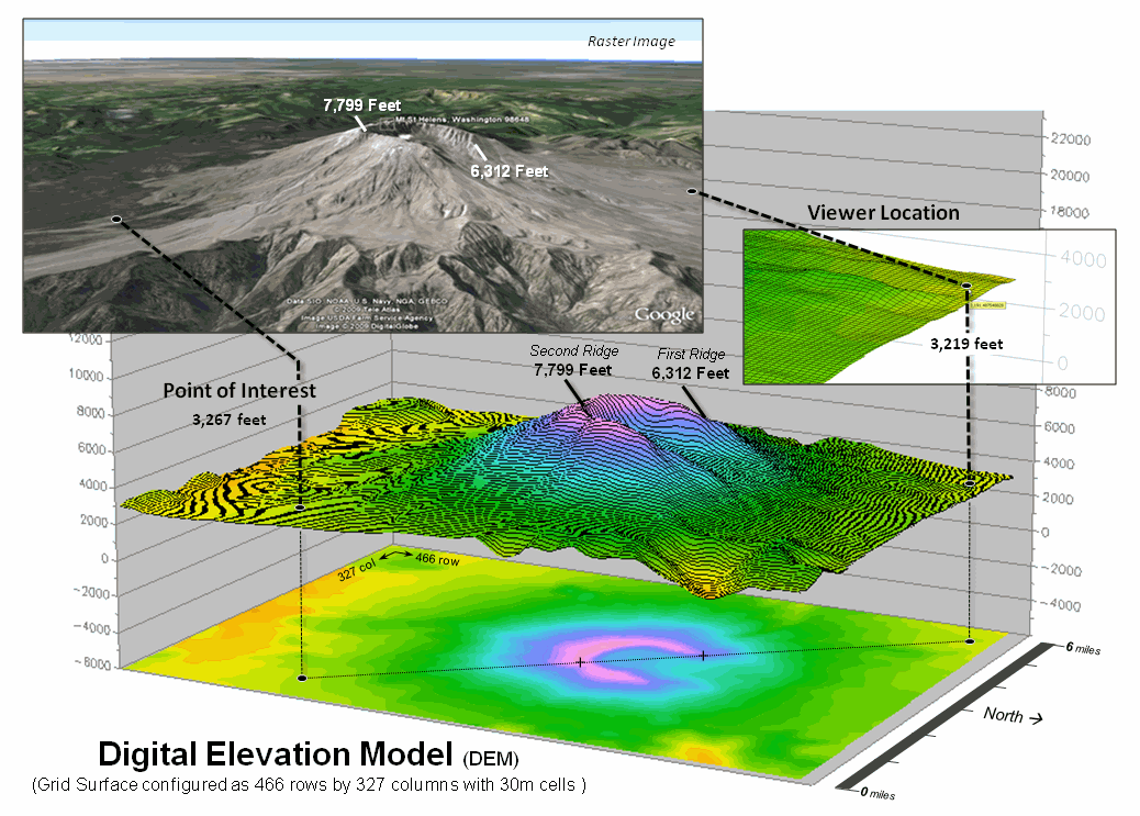
Figure 1. Mount St. Helens topography.

Underlying all this is a Digital Elevation Model (DEM) that encapsulates the topographic undulations. It uses traditional X and Y coordinates to position a location plus a Z coordinate to establish its relative height above a reference geode (sea level in this case). However from a purist’s perspective there are a couple of things that keep it from being a true three-dimensional GIS. First, the raster image is just that— a display in which thousands the “dumb” dots coalesce to form a picture in your mind, not an “intelligent” three-dimensional data structure that a computer can understand. Secondly, the rendering is still somewhat two-dimensional as the mapped information is simply “draped” on a wrinkled terrain surface and not stored in a true three-dimensional GIS—a warped pancake.

The DEM in the background forms Mt St. Helen’s three-dimensional terrain surface by storing elevation values in a matrix of 30 meter grid cells of 466 rows by 327 columns (152, 382 values). In this form, the computer can “see” the terrain and perform its map-ematical magic.

Figure 2 depicts a bit of computational gymnastics involving three-dimensional geography. Assume you are standing at the viewer location and looking to the southeast in the direction of the point of interest. Your elevation is 3,219 feet with the mountain’s western rim towering above you at 6,312 feet and blocking your view of anything beyond it. In a sense, the computer “sees” the same thing—except in mathematical terms. Using similar triangles, it can calculate the minimum point-of-interest height needed to be visibly connected as (see author’s notes for a link to discussion of the more robust “splash algorithm” for establishing visual connectivity)…

Tangent = Rise / Run

= (6312 ft – 3219 ft) / (SQRT[(134 – 33)² + (454 – 325) ² ] * 98.4251 ft)

= 3093 ft / (163.835 * 98.4251 ft) = 3893 ft / 16125 ft = 0.1918

Height = (Tangent * Run) + Viewer Height

= (0.1918 * (SQRT[(300 – 33)² + (454 – 114) ² ] * 98.4251 ft)) + 3219 ft

= (0.1918 * 432.307 * 98.4251 ft) + 3219 = 11,380 Feet

Figure 2. Basic geometric relationships determine the minimum visible height considering intervening ridges.

Since the computer knows that the elevation on the grid surface at that location is only 3,267 feet it knows you can’t see the location. But if a plane was flying 11,380 feet over the point it would be visible and the computer would know it.

Conversely, if you “helicoptered-up” 11,000 feet (to 14,219 feet elevation) you could see over both of the caldron’s ridges and be visually connected to the surface at the point of interest (figure 3). Or in a military context, an enemy combatant at that location would have line-of-sight detection.

As your vertical rise increases from the terrain surface, more and more terrain comes into view (see author’s notes for a link to an animated slide set). The visual exposure surface draped on the terrain and projected on the floor of the plot keeps track of the number of visual connections at every grid surface location in 1000 foot rise increments. The result is a traditional two-dimensional map of visual exposure at each surface location with warmer tones representing considerable visual exposure during your helicopter’s rise.

However, the vertical bar in figure 3 depicts the radical change that is taking us beyond mapping. In this case the two-dimensional grid “cell” (termed a pixel) is replace by a three-dimensional grid “cube” (termed a voxel)—an extension from the concept of an area on a surface to a glob in a volume. The warmer colors in the column identify volumetric locations with considerable visual exposure.

Figure 3. 3-D Grid Data Structure is a direct expansion of the 2D structure with X, Y and Z coordinates defining the position in a 3-dimensional data matrix plus a value representing the characteristic or condition (attribute) associated with that location.

Now imagine a continuous set of columns rising above and below the terrain that forms a three-dimensional project extent—a block instead of an area. How is the block defined and stored; what new analytical tools are available in a volumetric GIS; what new information is generated; how might you use it? …that’s fodder for the next section. For me, it’s a blast from the past that is defining the future of geotechnology.

____________________________

Author’s Notes: for a more detailed discussion of visual connectivity see the online book Beyond Mapping III, Topic 15, “Deriving and Using Visual Exposure Maps” at www.innovativegis.com/basis/MapAnalysis/Topic15/Topic15.htm. An annotated slide set demonstrating visual connectivity from increasing viewer heights is posted at www.innovativegis.com/basis/MapAnalysis/Topic27/AnimatedVE.ppt.

Thinking Outside the Box (pun intended)

(GeoWorld November, 2009)

Last section used a progressive series of line-of-sight connectivity examples to demonstrate thinking beyond a 2-D map world to a three-dimensional world. Since the introduction of the digital map, mapping geographic space has moved well beyond its traditional planimetric pancake perspective that flattens a curved earth onto a sheet of paper.

A contemporary Google Earth display provides an interactive 3-D image of the globe that you can fly through, zoom-up and down, tilt and turn much like Luke Skywalker’s bombing run on the Death Star. However both the traditional 2-D map and virtual reality’s 3-D visualization view the earth as a surface—flattened to a pancake or curved and wrinkled a bit to reflect the topography.

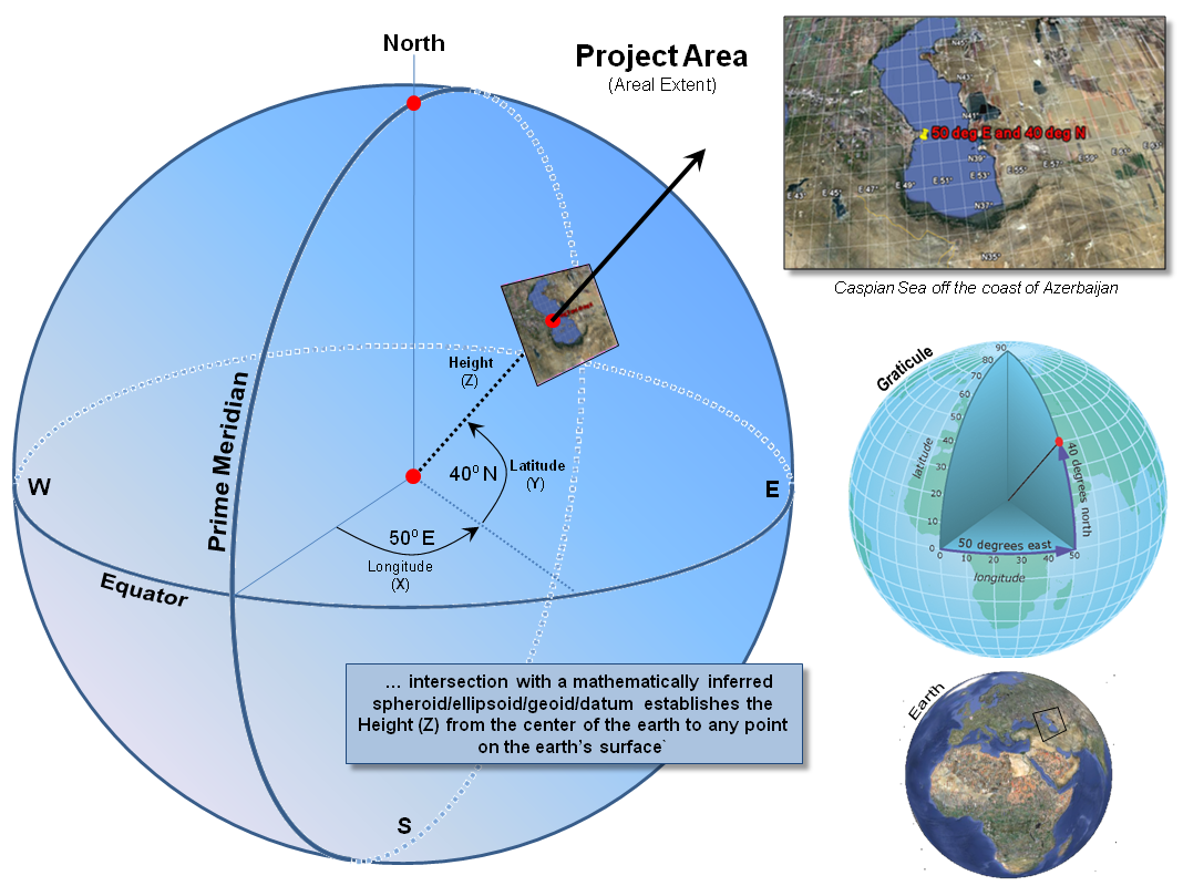
Figure 1. A 3-dimensional coordinate system uses angular measurements (X,Y) and length (Z) to locate points on the earth’s surface.

Figure 1 summarizes the key elements in locating yourself on the earth’s surface …sort of a pop-quiz from those foggy days of Geography 101. The Prime Meridian and Equator serve as base references for establishing the angular movements expressed in degrees of Longitude (X) and Latitude (Y) of an imaginary vector from the center of the earth passing through any location. The Height (Z) of the vector positions the point on the earth’s surface.

It’s the determination of height that causes most of us to trip over our geodesic mental block. First, the globe is not a perfect sphere but is a squished ellipsoid that is scrunched at the poles and pushed out along the equator like love-handles. Another way to conceptualize the physical shape of the surface is to imagine blowing up a giant balloon such that it “best fits” the actual shape of the earth (termed the geoid) most often aligning with mean sea level. The result is a smooth geometric equation characterizing the general shape of the earth’s surface.

But the earth’s mountains bump-up and valleys bump-down from the ellipsoid so a datum is designed to fit the earth's surface that accounts for the actual wrinkling of the globe as established by orbiting satellites. The most common datum for the world is WGS 84 (World Geodetic System 1984) used by all GPS equipment and tends to have and accuracy of +/- 30 meters or less from the actual local elevation anywhere on the surface.

The final step in traditional mapping is to flatten the curved and wrinkled surface to a planimetric projection and plot it on a piece of paper or display on a computer’s screen. It is at this stage all but the most fervent would-be geographers drop the course, or at least drop their attention span.

However, a true 3-D GIS simply places the surface in volumetric grid elements along with others above and below the surface. The right side of figure 2 shows a Project Block containing a million grid elements (termed “voxels”) positioned by their geographic coordinates—X (easting), Y (northing) and Z (height). The left side depicts stripping off one row of the elevation values defining the terrain surface and illustrating a small portion of them in the matrix by shading the top’s of the grids containing the surface.

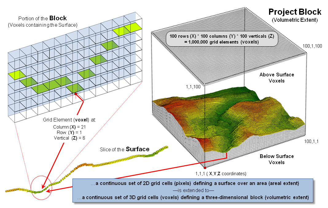
Figure 2. An implied 3-D matrix defines a volumetric Project Block, a concept analogous to areal extent in traditional mapping.

At first the representation in a true 3-D data structure seems trivial and inefficient (silly?) but its implications are huge. While topographic relief is stable (unless there is another Mount St. Helens blow that redefines local elevation) there are numerous map variables that can move about in the project block. For example, consider the weather “map” on the evening news that starts out in space and then dives down under the rain clouds. Or the National Geographic show that shows the Roman Coliseum from above then crashes through the walls to view the staircases and then proceeds through the arena’s floor to the gladiators’ hypogeum with its subterranean network of tunnels and cages.

Some “real cartographers” might argue that those aren’t maps but just flashy graphics and architectural drawings …that there has been a train wreck among mapping, computer-aided drawing, animation and computer games. On the other hand, there are those who advocate that these disciplines are converging on a single view of space—both imaginary and geographic. If the X, Y and Z coordinates represent geographic space, nothing says that Super Mario couldn’t hop around your neighborhood or that a car is stolen from your garage in Grand Theft Auto and race around the streets in your hometown.

The unifying concept is a “Project Block” composed of millions of spatially-referenced voxels. Line-of-sight connectivity determines what is seen as you peek around a corner or hover-up in a helicopter over a mountain. While the mathematics aren’t for the faint-hearted or tinker-toy computers of the past, the concept of a “volumetric map” as an extension of the traditional planimetric map is easy to grasp—a bunch of three-dimensional cubic grid elements extending up and down from our current raster set of squares (bottom of figure 3).

However, akin to the seemingly byzantine details in planimetric mapping, things aren’t that simple. Like the big bang of the universe, geographic space expands from the center of the earth and a simple stacking of fixed cubes like wooden blocks won’t align without significant gaps. In addition, the geometry of a cube does not have a consistent distance to all of its surrounding grid elements and of its twenty six neighbors only six share a complete side with the remaining neighbors sharing just a line or a single point. This inconsistent geometry makes a cube a poor grid element for 3-D data storage.

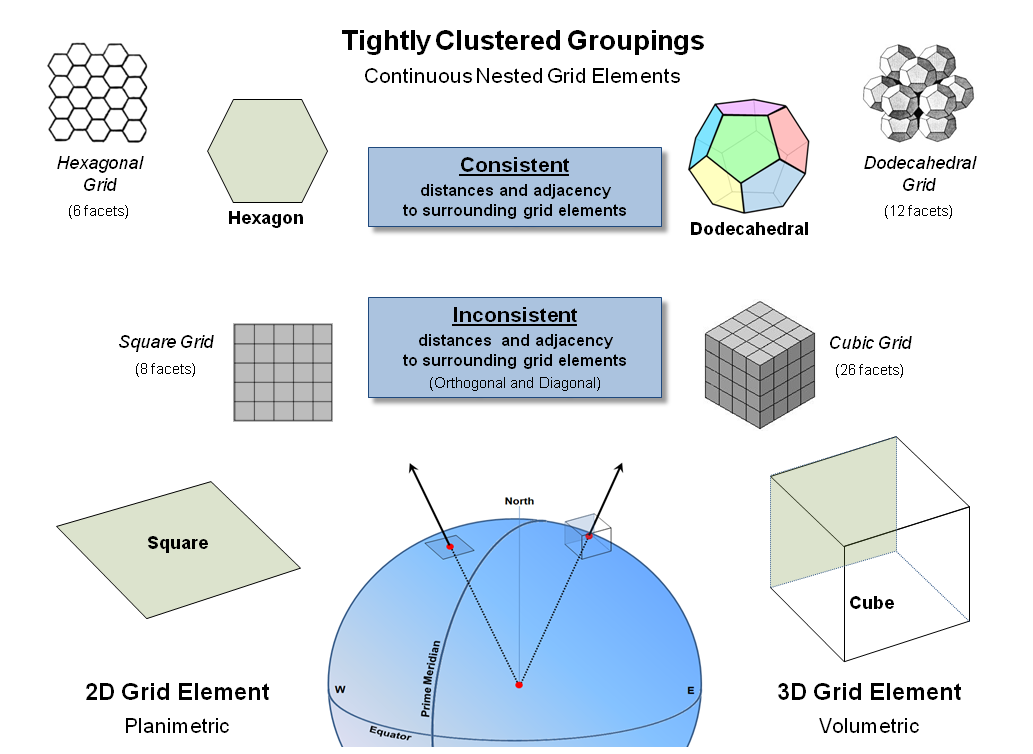
Figure 3. The hexagon and dodecahedral are alternative grid elements with consistent nesting geometry.

Similarly, it suggests that the traditional “square” of the Cartesian grid is a bit limited—only four complete sides (orthogonal elements) and four point adjacencies (diagonal). Also, the distances to surrounding elements are different (a ratio of 1:1.414). However, a 2D hexagon shape (beehive honey comb) abuts completely without gaps in planimetric space (termed “fully nested”); as does a combination of pentagon and hexagon shapes nests to form the surface of a spheroid (soccer ball).

To help envision an alternative 3-D grid element shape (top-right of figure 3) it is helpful to recall Buckminster Fuller's book Synergetics and his classic treatise of various "close-packing" arrangements for a group of spheres. Except in this instance, the sphere-shaped grid elements are replaced by "pentagonal dodecahedrons"— a set of uniform solid shapes with 12 pentagonal faces (termed geometric “facets”) that when packed abut completely without gaps (termed fully “nested”).

All of the facets are identical, as are the distances between the centroids of the adjoining clustered elements defining a very “natural” building block (see Author’s Note). But as always, “the Devil is in the details” and that discussion is dealt with in the next section.

_____________________________

Author’s Note: In 2003, a team of cosmologists and mathematicians used NASA’s WMAP cosmic background radiation data to develop a model for the shape of the universe. The study analyzed a variety of different shapes for the universe, including finite versus infinite, flat, negatively- curved (saddle-shaped), positively- curved (spherical) space and a torus (cylindrical).  The study revealed that the math adds up if the universe is finite and shaped like a pentagonal dodecahedron (http://physicsworld.com/cws/article/news/18368). And if one connects all the points in one of the pentagon facets, a 5-pointed star is formed.  The ratios of the lengths of the resulting line segments of the star are all based on phi, Φ, or 1.618… which is the “Golden Number” mentioned in the Da Vinci Code as the universal constant of design and appears in the proportions of many things in nature from DNA to the human body and the solar system—isn’t mathematics wonderful!

From a Mapping Pancake to a Soufflé

(GeoWorld November, 2009)

As the Time Traveller noted in H. G. Wells’ classic “The Time Machine,” the real world has three geometric dimensions not simply the two we commonly use in mapping. In fact, he further suggested that “...any real body must have extension in four directions: Length, Breadth, Thickness—and Duration (time)” …but that’s a whole other story.

Recall from last month’s column on 3D GIS that Geodetic Referencing (geographic position) used in identifying an “areal extent” in two-dimensions on the earth’s surface can be extended to a Database Referencing system (matrix location) effectively defining a 3-dimensional “project block” (see the left side of figure 1). The key is the use of Geodetic Height above and below the earth’s ellipsoid as measured along the perpendicular from the ellipsoid to provide the vertical (Z) axis for any location in 3-dimensional space.

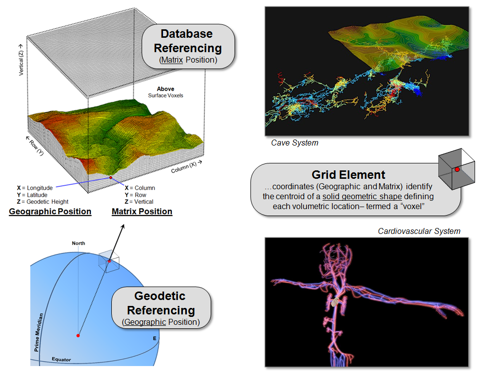
Figure 1. Storage of a vertical (Z) coordinate extends traditional 2D mapping to

3D volumetric representation.

The result is a coordinate system of columns (X), rows (Y), and verticals (Z) defining an imaginary matrix of grid elements, or “voxels,” that are a direct conceptual extension of the “pixels” in a 2D raster image. For example, the top-right inset in figure 1 shows a 3D map of a cave system using ArcGIS 3D Analyst software. The X, Y and Z positioning forms a 3-dimensional display of the network of interconnecting subterranean passages. The lower-right inset shows an analogous network of blood vessels for the human body except at much different scale. The important point is that both renderings are 3D visualizations and not a 3D GIS as they are unable to perform volumetric analyzes, such as directional flows along the passageways.

The distinction between 3D visualization and analytical systems arises from differences in their data structures. A 3D visualization system stores just three values—X and Y for “where” and Z for “what (elevation).” A 3-dimensional mapping system stores at least four values—X, Y and Z for “where” and an attribute value for “what” describing the characteristic/condition at each location within a project block.

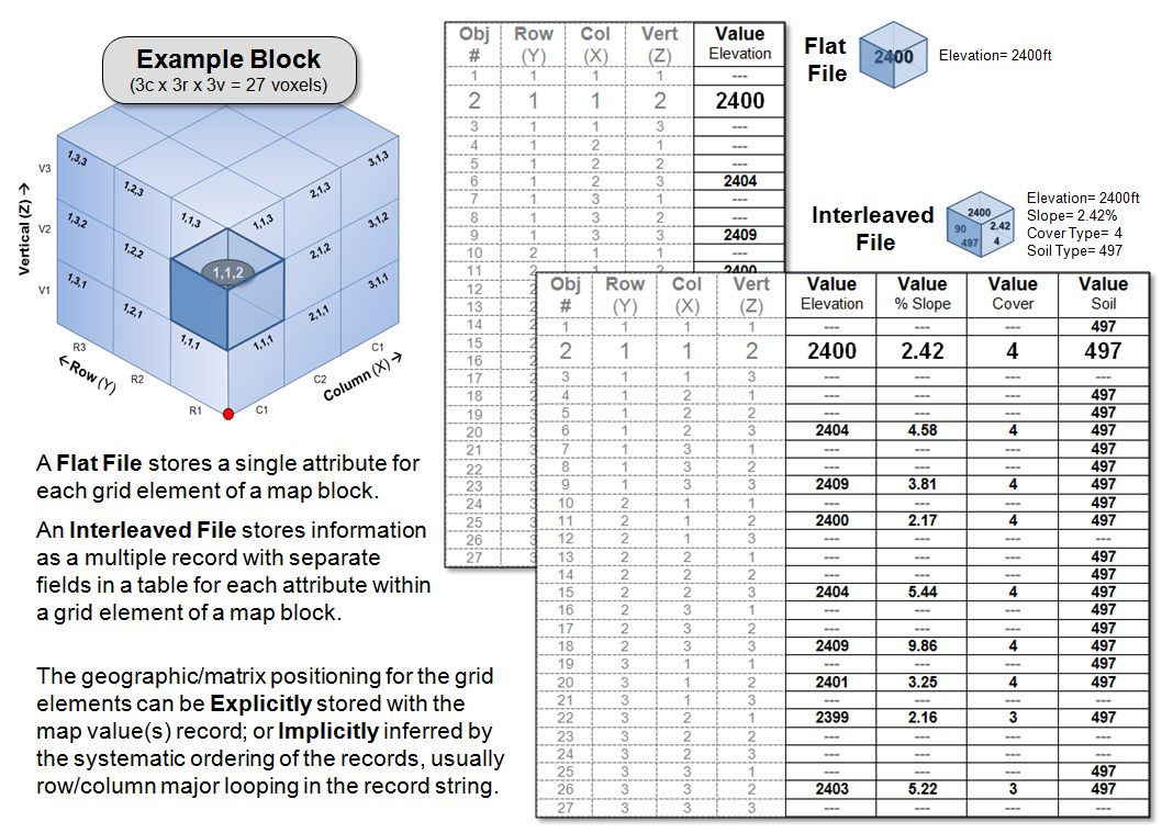
Figure 2. A 3-dimensional matrix structure can be used to organize volumetric mapped data.

Figure 2 illustrates two ways of storing 3-dimensional grid data. A Flat File stores a single map value for each grid element in a map block. The individual records can explicitly identify each grid element (grayed columns—“where”) along with the attribute (black column—“what”). Or, much more efficiently, the information can be implicitly organized as a header line containing the grid block configuration/size/referencing followed by a long string of numbers with each value’s position in the string determining its location in the block through standard nested programming loops. This shortened format provides for advanced compression techniques similar to those used in image files to greatly reduce file size.

An alternative strategy, termed an Interleaved File, stores a series of map attributes as separate fields for each record that in turn represents each grid element, either implicitly or explicitly organized into a table. Note that in the interleaved file in figure 2, the map values for Elevation, %Slope and Cover type identify surface characteristics with a “null value (---)” assigned to grid elements both above and below the surface. Soil type, on the other hand, contains values for the grid elements on and immediately below the surface with null values only assigned to locations above ground. This format reduces the number of files in a data set but complicates compression and has high table maintenance overhead for adding and deleting maps.

Figure 3 outlines some broader issues and future directions in 3D GIS data storage and processing. The top portion suggests that the inconsistent geometry of the traditional Cube results in differing distances and facet adjacency relationship to the surrounding twenty six neighbors, thereby making a cube a poor grid element for 3D data storage. A Dodecahedron, on the other hand, aligns with a consistent set of 12 equidistant pentagonal faces that “nest” without gaps ...an important condition in spatial analysis of movements, flows and proximal conditions.

The lower portion of figure 3 illustrates the knurly reality of geographic referencing in 3-dimensions—things change as distance from the center of the earth or bounding ellipsoid changes. Nicely nesting grid elements of a fixed size separate as distance increases (diverge); overlap as distance decreases (converge). To maintain a “close-packing” arrangement either the size of the grid element needs to adjust or the progressive errors of fixed size zones are tolerated.

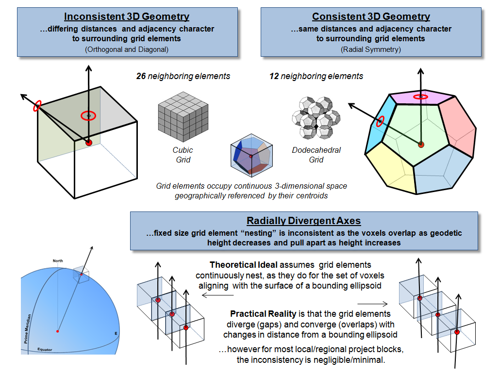
Figure 3. Alternative grid element shapes and new procedures for dealing with radial divergence

form the basis for continued 3D GIS research and development.

Similar historical changes in mapping paradigms and procedures occurred when we moved from a flat earth perspective to a round earth one that generated a lot of room for rethinking. There are likely some soon-to-be-famous mathematicians and geographers who will match the likes of the great Claudius Ptolemy (90-170), Gerardus Mercator (1512-1594) and Rene Descartes (1596-1650)— I wonder who among us will take us beyond mapping as we know it? Hopefully the advocates of a “flat mapping world” of discrete objects don’t have the same clout as Saint Augustine’s “flat earth” proponents; or the reach of the Spanish Inquisition enforcement arm.

_____________________________

Author’s Notes: A good discussion of polyhedral and other 3-dimensional coordinate systems is in Topic 12, “Modeling locational uncertainty via hierarchical tessellation,” by Geoffrey Dutton in Accuracy of Spatial Databases edited by Goodchild and Gopal. In his discussion he notes that “One common objection to polyhedral data models for GIS is that computations on the sphere are quite cumbersome … and for many applications the spherical/geographical coordinates … must be converted to and from Cartesian coordinates for input and output.”