Beyond Mapping
|
Map
Analysis book with companion CD-ROM for hands-on exercises and further reading |
GIS Software's
Changing Roles — discusses
the evolution of GIS software and identifies important trends
Determining Exactly
Where Is What
— discusses the
levels of precision and accuracy
Finding Common Ground
in Paper and Digital Worlds
— describes the
similarities and differences in information and organization between
traditional paper and digital maps
Resolving Map
Detail — discusses
the factors that determine the “informational scale” digital maps
Referencing
the Future — describes
current and alternative approaches for referencing geographic and abstract space
Is it Soup Yet? — describes
the evolution in definitions and terminology
What’s in a Name — suggests
and defines the new term Geotechnology
<Click here> right-click to download a
printer-friendly version of this topic (.pdf).
(Back
to the Table of Contents)
______________________________
(GeoWorld, September 1998, pg. 28-30)
Although
This point was struck home during a recent visit to Disneyland. The newest ride subjects you to a seemingly
endless harangue about the future of travel while you wait in line for over an
hour. The curious part is that the
departed Walt Disney himself is outlining the future through video clips from
the 1950s. The dream of futuristic
travel (application) hasn’t changed much and the 1990s practical reality
(tool), as embodied in the herky-jerky ride, is a long way from fulfilling the
vision.
What impedes the realization of a
technological dream is rarely a lack of vision, but the nuts and bolts needed
in its construction. In the case of
With the 1980s came the renaissance of modern computers and with it the
hardware and software environments needed by
Working within a
From an application developer’s perspective the floodgates had opened. From an end user’s perspective, however, a
key element still was missing—the gigabytes of data demanded by practical
applications. Once again
But another less obvious impediment hindered progress. As the comic strip character Pogo might say,
“…we have found the enemy and it’s us.”
By their very nature, the large
The 1990s saw both the data logjam burst and the
So where are we now? Has the role of
MapInfo’s MapX and ESRI’s MapObjects
are tangible
In its early stages,
The distinction between computer and application specialist isn’t so much their
roles, as it is characteristics of the combined product. From a user’s perspective the entire
character of a
As the future of
Determining Exactly Where Is
What
(GeoWorld, February 2008, pg. 14-15)
The Wikipedia defines Accuracy as “the degree of veracity” (exactness) while Precision as “the degree of
reproducibility” (repeatable). It uses
an archery target as an analogy to explain the difference between the two terms
where measurements are compared to arrows shot at the target (left side of
figure 1). Accuracy describes the
closeness of arrows to the bull’s-eye at the target center
(actual/correct). Arrows that strike
closer to the bullseye are considered more accurate.
Precision, on the
other hand, relates to the size of the cluster of several arrows. When the arrows are grouped tightly together,
the cluster is considered precise since they all strike close to the same spot,
if not necessarily near the bull’s-eye.
The measurements can be precise, though not necessarily accurate.
However, it is not
possible to reliably achieve accuracy in individual measurements without
precision. If the arrows are not grouped
close to one another, they cannot all be close to the bull’s-eye. While their average position might be an accurate estimation of the
bull’s-eye, the individual arrows are inaccurate.
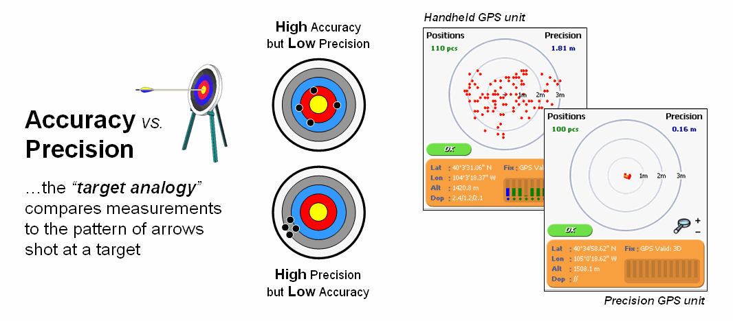
Figure
1. Accuracy refers to “exactness” and Precision
refers to “repeatability” of data.
So what does this
academic diatribe have to do with
In
Whereas
Figure 2
illustrates the two-fold consideration of Precise
Placement of coordinate delineation and Accurate
Assessment of attribute descriptor for three photo interpreters. The upper-right portion superimposes three
parcel delineations with Interpreter B outlining considerably more area than
Interpreters A and C—considerable variation in precision. The lower portion of the figure indicates
differences in classification with Interpreter B assigning Ponderosa pine as
the vegetation type—considerable variation in accuracy to the true Cottonwood
vegetation type correctly classified by Interpreters A and C.
Many

Figure
2. In mapped data, precision refers to placement
whereas accuracy refers to classification.
In addition, our
paper map legacy of visualizing maps frequently degrades precision/accuracy in
detailed mapped data. For example, a
detailed map of slope values containing decimal point differences in terrain
inclination can be easily calculated from an elevation surface. But the detailed continuous spatial data is
often aggregated into just a few discrete categories so humans can easily
conceptualize and “see” the information—such as polygonal areas of gentle,
moderate and steep terrain. Another
example is the reduction of the high precision/accuracy inherent in a
continuous “proximity to roads” map to that of a discrete “road buffer” map
that simply identifies all locations within a specified reach.
Further thought
suggests an additional consideration of
As you might
suspect, different groups have differing perspectives on the interpretation and
relative importance of the routing criteria.
For example, homeowners might be most concerned about Housing Density
and Visual Exposure; environmentalists most concerned about Road Proximity and
Sensitive Areas; and engineers most concerned about Housing Density and Road
Proximity. Executing the model for these
differences in perspective (relative importance of the criteria) resulted in
three different preferred routes.
The lower-left
portion of figure 3 shows the spread of the three individual solutions. One isn’t more precise/accurate
than another, just an expression of a particular perspective of the solution.
The lower-right side of the figure suggests yet another way to represent the
solution using the simple average of the three preference surfaces to identify
an overall route and its optimal corridor—sort of analogous to averaging a
series of
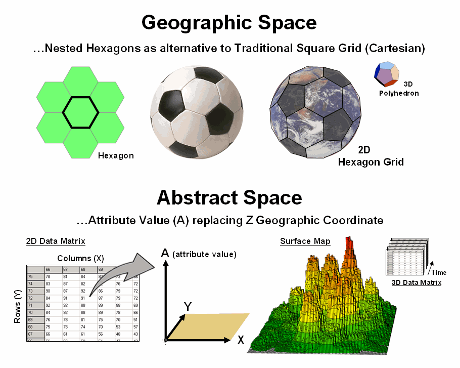
Figure 3. Maps derived by
The take home
from this discussion is that precision and accuracy is not the same thing and
that the terms can take on different meanings for different types of maps and
application settings. There are at least
three different levels of precision/accuracy—1) “Where is Where” considering just precise placement, 2) “Where is What”
considering placement and classification, and 3) “Where is What, if you assume…” considering placement,
classification and interpretation/logic/understanding/judgment ingrained in
spatial reasoning. Before
_____________________________
Author’s Notes: Related discussion of routing model considerations and procedures is in
Topic 8, Spatial Model Example in the book Map Analysis (Berry, 2007; GeoTec Media, www.geoplace.com/books/MapAnalysis) and Topic
19, Routing and Optimal Paths in the online Beyond Mapping
Finding Common Ground in Paper and
Digital Worlds
(GeoWorld, February 2007, pg. 28-30)
In the real world, landscapes are composed rocks, dirt, water, green stuff and furry/feathered friends. In a “paper world” these things are represented by words, tables and graphics. The traditional paper map is a graphical representation with inked lines, shadings and symbols used to locate landscape features using three basic building blocks— Points, Lines and Areas. For example, a typical water map might identify a well as a dot, a stream as a squiggle and a lake as a blue blob (figure 1). Each feature is considered a well-defined “discrete spatial object” with unique spatial character, positioning and dimension.

Figure 1. Traditional and Extended Map Features.
In geometry a point is considered dimensionless, however, the corresponding concept in cartography is a dot of ink having a physical dimension of a few inches to several miles depending on the scale of a paper map. Similarly, a line in mathematical theory has only length but is manually mapped as a thin serpentining polygon of the pen’s width. An area feature has both length and width in two-dimensional space. The interplay of mapping precision and accuracy in a digital world involves a discussion of scale and resolution reserved for the next section. For now, let’s consider the revolutionary changes in map form and content brought on by the digital map as outlined in the rest of figure 1.
For thousands of years, manual cartography has been limited to characterizing all geographic phenomena as discrete 2-dimensional spatial objects. However many map variables, such as elevation, change continuously and representation as contour lines suggests a nested series of flat layers like a wedding cake instead of the actual continuously undulating terrain. The introduction of a grid-based data structure provides for a new basic building block—a map Surface of continuously changing values throughout geographic space.
Another extension to the building blocks is Volumes that track length, width and depth in characterizing discrete or continuous variables in 3-dimensional space. For example, the L,W,D coordinates identify a specific location in a lake and a fourth value (attribute) can identify its temperature, turbidity, salinity or other condition.
A hyper-Volume (or hyper-point, -line, -area or -surface) introduces time as an additional abstract coordinate. For example, the weekly water volume of a reservoir might be tracked by L,W,D,T coordinates identifying a location in 3-dimensional space, as well as time combined with a fifth value indicating whether water is present or not. This conceptual extension is a bit tricky and provides discussion fodder about mixed referencing units (e.g., meters and minutes) for a later section. However, the result is a discrete volumetric map feature that shrinks and expands throughout a year—a dynamic spatial entity that at first appears to violate orthodox mapping commandments.
Another mind-bend brought on by the digital map is the concept of fuzzy-features. This idea tracks the certainty of a feature or condition at each map location. For example, the boundary line of a soil polygon is a subjective interpretation, while soil parcel’s actual edge could be a considerable distance away—“the boundary is likely here (high probability) but could be over there (low probability).” Another fuzzy example is a classified satellite image where statistical probabilities are used to establish which cover type is most likely.
Taken to the hilt, one can conceptualize a data structure that carries L,W,D,T and A,P (attribute and probability) descriptors that identify a location in space and time, as well as characterize its most likely condition, next most likely, and so on—sort of a sandwich of probable conditions. Such a representation challenges the infallible paradigm of mapping but opens a whole new world of error propagation modeling.
Whereas volumes, hyper-volumes and fuzzy-features define the current realm of GIS researchers, an understanding of contemporary approaches for characterizing points, lines, and areas is necessary for all GIS users. Figure 2 outlines the two fundamental approaches—vector and raster (see Author’s Notes).
A Point defined by X,Y coordinates in vector, and a Cell defined by Col,Row indices in raster, form the basic data structure units—the “smallest addressable unit of space” in a map. Lines are formed by mathematically connecting points (vector) or identifying all of the conjoined cells containing a line (raster). Areas are defined by a set of points that define a closed line encompassing a feature (vector) or by all of the contiguous cells containing a feature (raster).
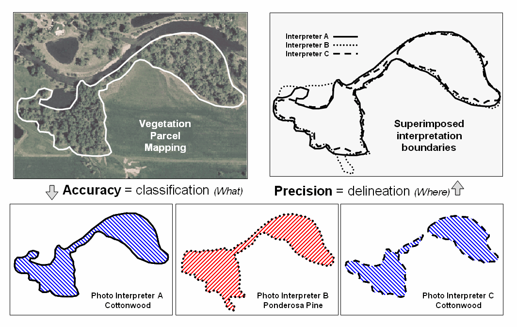
Figure 2. Basic Vector and Raster Data Structure Considerations.
While spatial precision is a major operational difference between vector and raster systems, how they characterize geographic space is important in understanding limitations and capabilities. Vector precisely identifies critical points along a line, but the intervening connections are implied. Raster, on the other hand, identifies all of the cells containing a line without any implied gaps. Similarly, vector precisely stores an area’s boundary but implies its interior (must calculate); raster stores the interior but implies the boundary (must calculate).
The differences in “what is defined” and “what is implied” determine just about everything in GIS technology, except maybe the color pallet for display—data structure, storage requirements, algorithms, coding and ultimately appropriate use. Vector systems precisely and efficiently store traditional discrete map objects, such as underground cables and property boundaries (mapping and inventory). Raster systems, on the other hand, predefine continuous geographic space for rapid and enhanced processing of map layers (analysis and modeling).
So how do you think vector and raster systems store surfaces, volumes, hyper-volumes and fuzzy-features? …very poorly, or not at all for vector systems. However raster systems pre-define all of a project area (no gaps) by carrying a thematic value for each cell in a 2-dimensional storage matrix to form a continuous map surface. For volumes, a third geographic referencing index is added to extend the 2D cells to 3D cubes in geographic space defined by their X,Y,Z position in the storage matrix see Author’s Notes).
A similar expansion is used for hyper-volumes with four indices (X,Y,Z,T) identifying the “position,” except in this instance an abstract space is implied due to the differences in geographic and time units. Information about fuzzy-features can be coded into a compound attribute value describing any map feature, where the first few digits identify the character/condition at a location with the trailing two digits identifying the certainty of classification.
The bottom line is that tomorrow’s maps aren’t simply colorful electronic versions of your grandfather’s maps. The digital map is an entirely different beast supporting radically new mapping approaches, perspectives, opportunities and responsibilities.
_____________________________
Author’s Notes: Topic 6, “Alternative Data Structures,” in Spatial
Reasoning for Effective GIS (Berry 1995, Wiley) contrasts vector and raster
data structures and describes related alternative structures including TIN, Quadtree, Rasterized Lines and Vectorized Cells.
(GeoWorld, March 2007, pg. 28-30)
One of the most fundamental concepts in the paper map world is Geographic Scale—the relationship between a distance on a map and its corresponding distance on the earth. In equation form, scaleratio= map distance / ground distance but is often expressed as a representative fraction (RF), such as scaleRF= 1:63,360 meaning 1 inch on the map represents 63,360 inches (or 1 mile) on the earth’s surface.
However in the digital map world, this traditional concept of scale does not exist. While at first this might seem like cartographic heresy, note that the “map distance” component of the relationship is assumed to be fixed as ink marks on paper. In a GIS, however, the map features are stored as organized sets of numbers representing their spatial position (coordinates for “where”) and thematic attribute (map values for “what”). One can zoom in and out on the data thereby creating a continuous gradient of geographic scales in the resulting display or hardcopy plot.
Hence geographic scale is a function of the display, not an inherent property of the digital mapped data set. What is important is the implied concept of informational scale, or Resolution—the ability to discern detail. Traditionally it is implicit that as geographic scale decreases, resolution also diminishes since drafted feature boundaries must be smoothed, simplified or not shown at all due to the width of the inked lines.
Figure 1. Spatial Resolution describes the level of positional detail used to
track a geographic pattern or distribution.
However in a GIS, the concept of resolution is explicit. In fact there are five types of resolution that need to be considered—Spatial, Map, Thematic, Temporal and Model. Spatial Resolution is the most basic and identifies the “smallest addressable unit” of geographic space (figure 1). For point features, the X,Y coordinates (vector) and cell size (raster) determine the smallest addressable unit.
For line features in vector, however, the smallest addressable unit is the line segment with larger segments capturing less detail as the implied straight line misses the subtle wiggles and waggles of a pattern. Similarly, large grid cells capture less linear detail than smaller cells.
For polygon features in vector, an entire polygon represents the smallest addressable unit as the boundary needs to be completed before the implied interior condition can be identified. In raster, the smallest addressable unit is defined by the cell size as the condition is carried for each of the cells comprising the interior and edge of a polygon feature.
The concept of spatial resolution easily extends to the level of spatial aggregation or Map Resolution that identifies the “smallest physical grouping” of a map theme (figure 2). For example, a high resolution forest map might identify individual trees (very small polygons delineating canopy extent), whereas more generally, numerous trees are used to identify a forest parcel of several acres that ignores the scattered tree occurrences. The size of the minimum polygon is determined by the interpretation process with smaller groupings capturing more detail of the pattern and distribution.
Figure 2. Map Resolution describes the level of physical aggregation used to
depict a geographic pattern or distribution.
Thematic Resolution identifies the “smallest classification grouping” of a map theme. For example, a simple forest/non-forest map might provide a sufficient description of vegetation for some uses and this coarse classification has appeared for years as green on USGS topographic sheets. However, resource managers require a higher thematic resolution of vegetation cover and expand the classification scheme to include species, age, stocking level and other characteristics. The result is a finer classification categories of a generalized forest area into smaller more detailed parcels (figure 3).
A forth consideration involves Temporal Resolution that identifies the frequency, or time-step of map update. Some data types, such as geological and landform maps, change very slowly and do not need frequent revision. A city planner, on the other hand, needs land use maps that are updated every couple of years and include future development sites. A retail marketer needs even higher temporal resolution and will likely update sales and projection figures on a monthly, weekly or even daily basis.
Model Resolution is the least defined and involves factors affecting the level of detail used in creating a derived map, such as an optimal corridor for an electric transmission line or areas of suitable wildlife habitat. Model resolution considers detail ingrained in 1) the interpretation/analysis assumptions (logic) and 2) the algorithms/procedures (processing) used in implementing a spatial model. For example, a proposed transmission line could be routed considering just terrain steepness for a low model resolution, or extended to include other engineering factors (soils, road proximity, etc.), environmental concerns (wetlands, wildlife habitats, etc.) and social considerations (visual exposure, housing density, etc.) for much higher model resolution.
Figure 3. Thematic Resolution describes the level of classification aggregation
used to depict a geographic pattern or distribution.
So why should we care about digital map resolution? Because accounting for informational scale is just as important as adjusting for a common geographic scale and projection when interacting with a stack of maps. Our paper map heritage focused on descriptive mapping (inventory of physical phenomena) whereas an increasing part of the GIS revolution focuses on prescriptive mapping (spatial relationships of physical and cognitive interactions). This “thinking with maps” requires a thorough understanding of the spatial, map, thematic, temporal and model resolutions of the maps involved or you will surely be burned.
(GeoWorld, April 2007, pg. 28-30)
Geo-referencing is the cornerstone of GIS. In the mid-1600s the French mathematician, René Descartes established the Cartesian
coordinate system that is still in use today.
The system determines the
location of each point in a plane as defined by two numbers—a x-coordinate and a y-coordinate.
A third z-coordinate is used to extend the system
to 3-dimensional geographic space (see Author’s Notes). In mapping, these coordinates reference a
refined ellipsoid (geodetic datum) that can be conceptualized as a curved surface approximating the mean ocean
surface of the earth.
The location and
shape of map features can be established by X and Y distances measured along
flattened portions of the reference surface (figure 1). The familiar Universal Transverse
Mercator (UTM) coordinates represent
E-W and N-S movements in meters along the plane. The rub is that UTM zones are need to break
the curved earth surface into a series of small flat, projected subsections
that are difficult to edge-match.
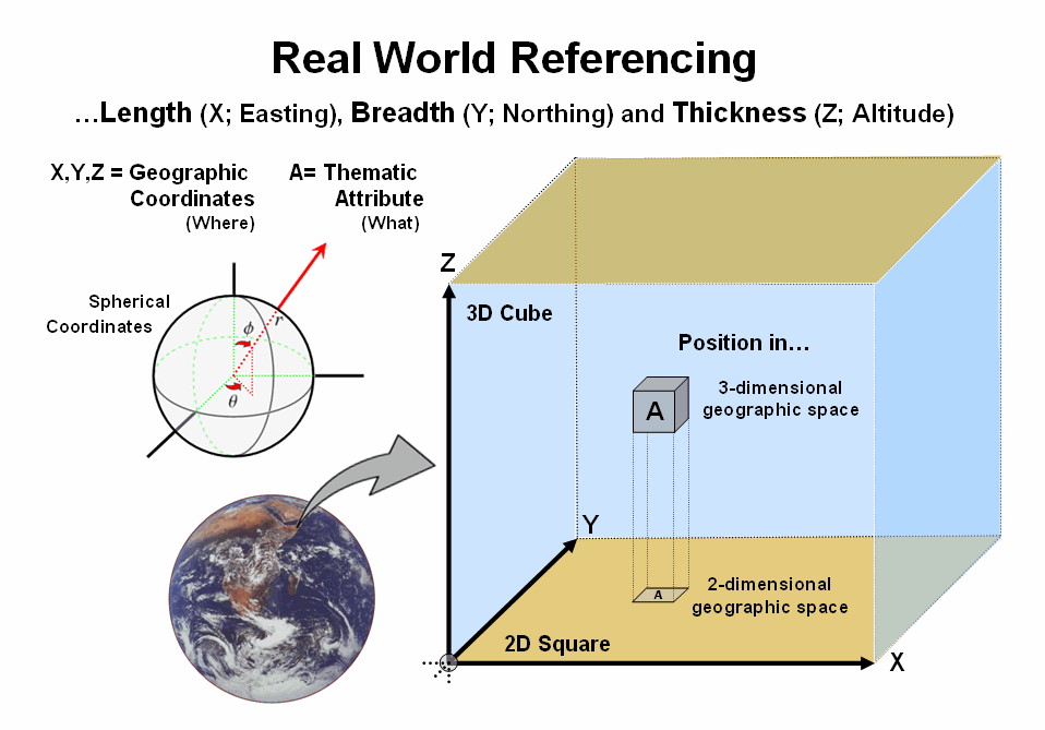
Figure 1. Geographic referencing uses three coordinates to locate map features
in real world space.
A variant of the traditional referencing system uses spherical coordinates that are based on solid angles measured from the center of the earth. This natural form for describing positions on a sphere is defined by three coordinates—an azimuthal angle (θ) in the X,Y plane from the x-axis, the polar angle (φ) from the z-axis, and the radial distance (r) from the earth’s center (origin). The advantage of a spherical referencing system is that it is seamless throughout the globe and doesn’t require projecting to a localized flat plane.
Digital map storage is rapidly moving toward spherical referencing that
uses latitude and longitude in decimal degrees for internal storage and
on-the-fly conversion to any planar projection.
This radical change from our paper map heritage is fueled by ubiquitous use of GPS and a desire for
global databases that easily walk across political and administrative
boundaries.
Since the digital
map is a radical departure from the paper map, other alternative referencing
schemes are possible. For example,
hexagons can replace the Cartesian grid squares we have used for hundreds of
years (top portion of figure 2). The
hexagon naturally nests to form a continuous network like a beehive’s
honeycomb. An important property of a
hexagon grid is that it better represents curved surfaces than a square grid— a
soccer ball stitched from squares wouldn’t roll the same [Note: actually a soccer ball is a composite of hexagons (white) and
pentagons (black)].
However the most
important property is that a hexagon has six sides instead of four. The added directions provide a foothold for
more precise measurement of continuous movement— one can turn right- and
left-oblique as well as just right and left.
Traditional routing models using Least Cost Path would benefit greatly.
Expanding to 3-dimensional geographic space provides for polyhedrons to replace cubes. For example, a dodecahedron is a nesting twelve-sided object that can be used instead of the six-sided cube. Weather and ground water flow modeling could be greatly enhanced by the increased options for transfer from a location to its larger set of adjoining locations. The computations for cross-products of vectors, such as warp-speed cruise missiles, could be greatly assisted as they are affected by different atmospheric conditions and evasive trajectories.

Figure 2. Alternative referencing systems
and abstract space characterization are possible through the digital nature of
modern maps.
Another extension involves the use of abstract space (bottom portion of figure 2). For example, the Z-coordinate can be replaced with an attribute value to generate a map surface, such as customer density. In this instance, the abstract referencing is a mixture of spatial and attribute “coordinates” and doesn’t imply 3-dimensional, real word geographic occurrences. Instead, it relates geography and conditions in an extremely useful way for conceptualizing patterns. Normalization along the abstract coordinate axis is an important consideration for both visualization and analysis.
This brings us to space-time referencing. During a recent panel discussion I was challenged for suggesting such a combination is possible within a GIS. The idea has been debated for years by philosophers and physicists but H.G. Wells’ succinct description is one of the best—
'Clearly,' the Time Traveller proceeded, 'any real body must have extension in
four directions: it must have Length, Breadth, Thickness, and - Duration. But
through a natural infirmity of the flesh, which I will explain to you in a
moment, we incline to overlook this fact. There are really four dimensions,
three which we call the three planes of Space, and a fourth, Time. There is,
however, a tendency to draw an unreal distinction between the former three
dimensions and the latter, because it happens that our consciousness moves
intermittently in one direction along the latter from the beginning to the end
of our lives.' (Chapter 1, Time Machine).
The upshot seems to be that a fourth dimension exists (see Author’s Notes), it is just you can’t go there in person. But a GIS can easily take you there—conceptually that is. For example, an additional abstract “coordinate” representing time can be added to form a 3-dimensional data matrix. The GIS picks off the customer density data for the first “page” and displays it as in the figure. Then it uses the data on the on the second page (one time step forward) and displays it. This is repeated to cycle through time and you see an animation where the peaks and valleys of the density surface move with time.
So animation enables you to move around a city (X,Y) viewing the space-time relationship of customer density (A). In a similar manner you could evaluate a forest “green-up” model to predict re-growth at a series of time steps after harvesting to look into future landscape conditions. Or you can watch the progression over time of ground water pollutant flow in 3D space (4D data matrix) using a semi-transparent dodecahedron solid grid just for fun and increased modeling accuracy. In fact, it can be argued that GIS is inherently n-dimensional when you consider a map stack of multiple attributes and time is simply another abstract dimension.
My suspicions are that revolutions in referencing will be a big part of GIS’s frontier in the 2010s. See you there?
_____________________________
Author’s Notes: an
excellent online reference for the basic geometry concepts underlying
traditional and future geo-referencing techniques is the Wolfram MathWorld pages, such as the posting describing the dodecahedron at http://mathworld.wolfram.com/Dodecahedron.html;
a
Is it Soup Yet?
(GeoWorld, February 2009)
In the forty-odd years of computer-tinkering with maps our perspectives and terminologies have radically changed. My first encounter was in the late 1960s as an undergraduate research assistant at the University of California, Berkeley. The entry point was through photogrammetric interpretation in the pursuit of a high resolution contour map for the school’s forest. In those days one stared at pair of stereo-matched aerial photos and marched a dot at a constant elevation around the three-dimensional surface that appeared. The result was an inked contour line drawn by a drafting arm that was mechanically connected to the stereo plotter— raise the dot and re-walk to delineate the next higher contour line.
The research effort took this process to a new level by augmenting the mechanical arm with potentiometers that converted the movements of the arm into X,Y coordinates that, in turn, were recorded by direct entry into a keypunch machine. After several months of tinkering with the Rube Goldberg device several boxes of punch cards were generated containing the digital representation of the contour lines that depicted the undulating shape of the terrain surface.
The card boxes then were transferred to a guru who ran the only large-bed plotter on campus and after a couple of more months of tinkering the inked lines emerged. While far from operational, the research crossed a technological threshold by replacing the analog mechanics of traditional drafting with the digital encoding required to drive the cold steel arm of a plotter—maps were catapulted from drawings to organized sets of numbers.
In the 1970’s Computer Mapping emerged through the efforts of several loosely allied fields involved in mapping—geography for the underlying theory, computer science for the software, engineering for the hardware and several applied fields for the practical applications. As depicted in figure 1, some of the more important perspectives and definitions of the emerging technology at that time were:
-
Surveying is the technique and science of accurately determining
the terrestrial or three-dimensional space position of points and the distances
and angles between them where these points are usually, but not exclusively,
associated with positions on the surface of the Earth, and are often used to
establish land maps and boundaries for ownership or governmental purposes. (Wikipedia
definition)
-
Photogrammetry is the first remote sensing technology ever
developed, in which geometric properties about objects are determined from
photographic images. (Wikipedia definition)
-
Remote Sensing is the small or
large-scale acquisition of information of an object or phenomenon, by the use
of either recording or real-time sensing device(s) that is not in physical or
intimate contact with the object (such as by way of aircraft, spacecraft,
satellite, etc.). (Wikipedia definition)
-
Computer-aided Drafting and Computer-assisted Mapping (CAD/CAM) is
the mapping expression of Computer-aided Design that uses computer technology to aid in the design and
particularly the drafting (technical drawing and engineering drawing) of a part
or product. (Wikipedia
definition)
-
Automated Cartography is the process of producing maps with the aid of
computer driven devices such as plotters and graphical displays. (Webopedia definition)
-
Image processing is any form of signal processing
for which the input is an image, such as photographs or frames of video with
the output of image processing being either an image or a set of
characteristics or parameters related to the image. (Wikipedia
definition)
The common thread at the time was an inspiration to automate the map drafting process by exploiting the new digital map form. The focus was on the graphical rendering of the precise placement of map features—an automated means of generating traditional map products. For example, the boxes of cards containing the contour lines of research project were mothballed after the plotter generated the printer’s separate used for printing multiple copies of the map.
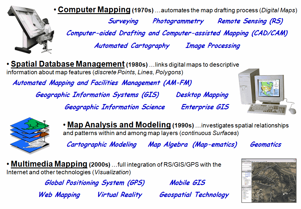
Figure
1. The
terminology and paradigm trajectory of GIS’s evolution.
Spatial Database Management expanded this view in the 1980s by combining the digital map coordinates (Where) with database attributes describing the map features (What). The focus shifted to the digital nature of mapped data and the new organizational capabilities it provided. Some of the perspectives and terms associated with the era were:
-
Automated Mapping and Facilities Management (AM-FM) seeks
to automate the mapping process and to manage facilities represented by items
on the map. (GITA definition)
-
Geographic Information System (GIS) is an information system for
capturing, storing, analyzing, managing and presenting data which are spatially
referenced (linked to location). (Wikipedia definition)
-
Geographic Information Science (GISc or GISci)
is the academic theory behind the development, use, and application of
geographic information systems (GIS). (Wikipedia definition)
-
Desktop Mapping involves using a desktop computer to perform
digital mapping functions. (eNCYCLOPEDIA definition)
-
Enterprise GIS is a platform for delivering organization-wide
geospatial capabilities providing for the free flow of information. (ESRI definition)
Geo-query became
the rage and organizations scurried to integrate their paper maps and
management records for cost savings and improved information access. The overriding focus was on efficient
recordkeeping, processing and information retrieval. The approach linked discrete Point, Line and Polygon features to database records
describing the spatial entities.
Map Analysis and Modeling in the 1990s changed the traditional mapping paradigm by introducing a new fundamental map feature—the continuous Surface. Some of the more important terms and perspectives of that era were:
-
Cartographic Modeling is a process that
identifies a set of interacting, ordered map operations that act on raw data,
as well as derived and intermediate data, to simulate a spatial decision making
process. (Tomlin definition)
-
Map Algebra (and Map-ematics)
is a simple
and an elegant set-based algebra for manipulating geographic data where the
input and output for each operator is a map and the operators can be combined
into a procedure to perform complex tasks. (Wikipedia definition)
-
Geomatics incorporates the older
field of surveying along with many other aspects of spatial data management
which integrates acquisition, modeling, analysis, and management of spatially
referenced data. (Wikipedia definition)
While much of the map-ematical theory and procedures
were in place much earlier, this era saw a broadening of interest in map
analysis and modeling capabilities. The
comfortable concepts and successful extensions of traditional mapping through
Spatial Database Management systems lead many organizations to venture into the
more unfamiliar realms of spatial analysis and statistics. The emerging applications directly infused
spatial considerations into the decision-making process by expanding “Where is What?” recordkeeping to “Why, So
What and What If?” spatial reasoning—thinking with maps to solve complex
problems.
Multimedia Mapping in
the 2000s turned the technology totally on its head by bringing it to the
masses. Spurred by the proliferation of
personal computers and Internet access, spatial information and some “killer
apps” have redefined what maps are, how one interacts with them, as well as
their applications. Important terms and
perspectives of the times include:
-
Global Positioning System (GPS) is the only fully functional
Global Navigation Satellite System (GNSS) that enable GPS receivers to
determine their current location, the time, and their velocity. (Wikipedia
definition)
-
Mobile GIS is the use of geographic data in the field on mobile
devices that integrates three essential components— Global Positioning System
(GPS), rugged handheld computers, and GIS software. (Trimble
definition)
-
Web Mapping is the process of designing, implementing,
generating and delivering maps on the World Wide Web. (Wikipedia
definition)
-
Virtual Reality (VR) is a technology which allows a user
to interact with a computer-simulated environment, be it a real or imagined
one. (Wikipedia
definition)
-
Geospatial Technology refers to technology used for
visualization, measurement, and analysis of features or phenomena that occur on
the earth that includes three different technologies that are all related to
mapping features on the surface of the earth— GPS (global positioning systems),
GIS (geographical information systems), and RS (remote sensing). (Wikipedia
definition)
The technology
has assumed a commonplace status in society as people access real-time driving
directions, routinely check home values in their neighborhood and virtually “fly”
to anyplace place on the earth to view the surroundings or checkout a
restaurant’s menu. While spatial
information isn’t the driver of this global electronic revolution, the
technology both benefits from and contributes to its richness. What was just a gleam in a handful of
researchers’ eyes thirty years ago has evolved into a pervasive layer in the
fabric of society, not to mention a major industry.
But what are the
perspectives and terms defining the technology’s future? That’s ample fodder for the next section.
_____________________________
Author’s Notes: a brief White
Paper describing GIS’s evolution is posted online at www.innovativegis.com/basis/Papers/Other/Geotechnology/Geotechnology_history_future.htm
. An interesting and useful Glossary of
GIS terms by Blinn, Queen and Maki of the University of
Minnesota is posted at www.extension.umn.edu/distribution/naturalresources/components/DD6097ag.html.
What’s in a Name
(GeoWorld, March 2009)
The previous section traced the evolution of modern mapping by identifying some of the more important labels and terminology that have been used to describe and explain what is involved. In just four decades, the field has progressed from an era of Computer Mapping to Spatial Database Management, then to Map Analysis and Modeling and finally to Multimedia Mapping.
The perspective of the technology has expanded from simply automated cartography to an information science that links spatial and attribute data, then to an analytical framework for investigating spatial patterns/relationships and finally to the full integration of the spatial triad of Remote Sensing (RS), Geographic Information Systems (GIS) and the Global Positioning System (GPS) with the Internet and other applied technologies.
While the evolution is in large part driven by technological advances, it also reflects an expanding acceptance and understanding by user communities and the general public. In fact, the field has matured to a point where the US Department of Labor has identified Geotechnology as “one of the three most important emerging and evolving fields, along with nanotechnology and biotechnology” (see Author’s Notes). This is rare company indeed.
The Wikipedia defines Biotechnology as “any technological application that uses biological systems, living organisms, or derivations thereof, to make or modify products or processes for specific use,” and Nanotechnology as “a field whose theme is the control of matter on and atomic and molecular scale.” By any measure these are sweeping definitions that encompass a multitude of sub-disciplines, conceptual approaches and paradigms. Figure 1 suggests a similar sweeping conceptualization for Geotechnology.
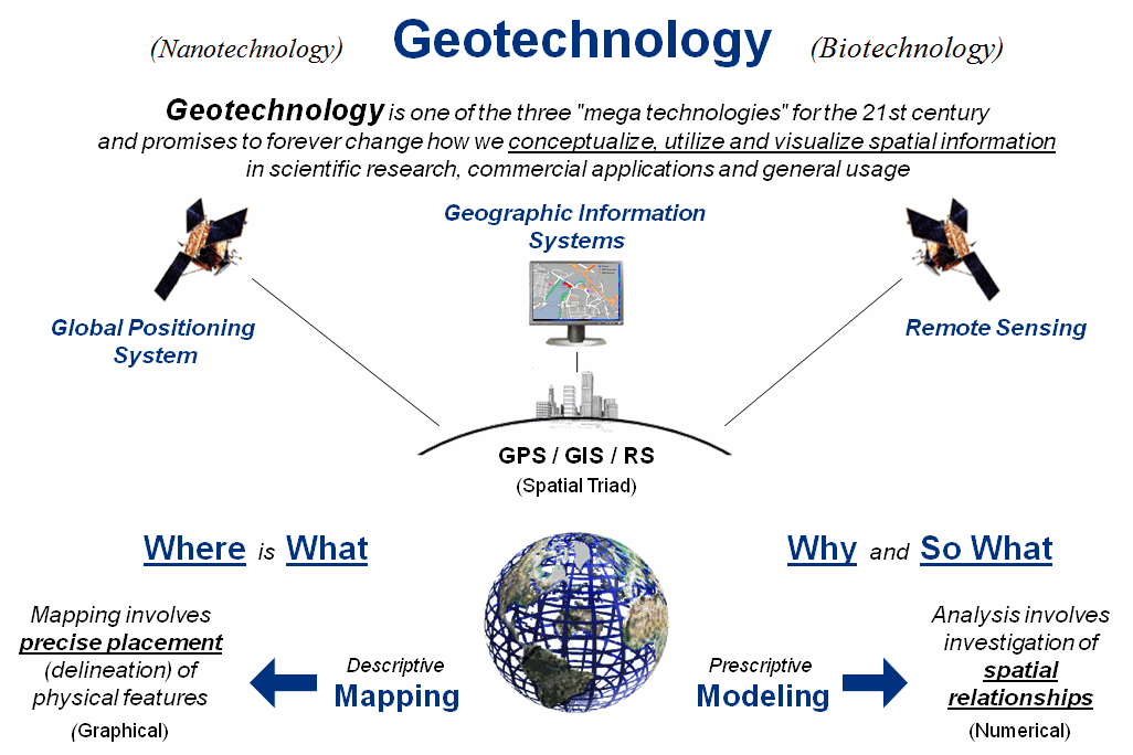
Figure 1. Conceptual framework of Geotechnology.
The top portion
of the figure relates Geotechnology to “spatial information” in a broad stroke
similar to biotechnology’s use of “biological systems” and nanotechnology’s use
of “control of matter.” The middle
portion identifies the three related technologies for mapping features on the
surface of the earth— GPS, GIS and RS.
The bottom portion identifies the two dominant application arenas that
emphasize descriptive Mapping (Where
is What) and
prescriptive Modeling (Why and So What).
What is most
important to keep in mind is that geotechnology, like bio- and nanotechnology, is
greater than the sum of its parts—GPS, GIS and RS. While these individual mapping technologies
provide the enabling capabilities, it is the application environments
themselves that propel geotechnology to mega status. For example, precision agriculture couples
the spatial triad with robotics to completely change crop production. Similarly, coupling “computer agents” with
the spatial triad produces an interactive system that has radically altered
marketing and advertising through spatially-specific queries and displayed
results. Or coupling immersive
photography with the spatial triad to generate an entirely type of “street
view” map that drastically changes 8,000 years of analog mapping.
To this point in
our technology’s short four decade evolution it has been repeatedly defined
from within. The
current “geospatial technology” moniker focuses on the interworking parts that
resonates with GIS specialists (see figure 2). However to the uninitiated, the term is as
off-putting as it is confusing—geo (Latin
for the earth), spatial (pertaining
to space), technology (application
of science). Heck, it even sounds redundant and is almost
as introvertedly-cute as the terms geomatics and map-ematics.
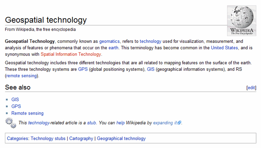
Figure 2. Wikipedia Definition of Geospatial Technology.
On the other
hand, the use of the emerging term “Geotechnology” for the first time provides
an opportunity to craft a definition with a broader perspective that embraces
the universality of its application environments and societal impacts along the
lines of the bio- and nanotechnology definitions.
As a draft
attempt, let me suggest—
Geotechnology refers to any
technological application that utilizes spatial location in visualizing,
measuring, storing, retrieving, mapping and analyzing features or phenomena
that occur on, below or above the earth.
It is recognized by the U.S. Department of Labor as one of the “three
mega-technologies for the 21st Century,” along with Biotechnology
and Nanotechnology. There are three
primary mapping technologies that enable geotechnology— GPS (Global Positioning
System), GIS (Geographic Information Systems) and RS (Remote Sensing). …etcetera, etcetera, etcetera… to quote
a famous King of Siam.
As with any controversial endeavor, the devil is in the details (the etcetera). One of the biggest problems with the term is that geology staked the flag several years ago with its definition of geotechnology as “the application of the methods of engineering and science to exploitation of natural resources” (yes, they use the politically incorrect term “exploitation”). Also, there is an International Society for Environmental Geotechnology, as well as a several books with the term embedded in their titles.
On the bright side, the Wikipedia doesn’t have an entry for Geotechnology. Nor is the shortened term “geo” exclusive to geology; in fact just the opposite, as geography is most frequently associated with the term (geo + graph + y literally means “to write the descriptive science dealing with the surface of the earth”). Finally, there are other disciplines, application users and the general public that are desperate for an encompassing term and succinct definition of our field that doesn’t leave them tongue-tied, shaking their heads in dismay or otherwise dumbfounded.
Such is the byzantine fodder of academics …any inspired souls out there willing to take on the challenge of evolving/expanding the definition of Geotechnology, as well as the perspective of our GPS/GIS/RS enabled mapping technology?
_____________________________
Author’s Notes: see www.nature.com/nature/journal/v427/n6972/full/nj6972-376a.html for an
article in Nature (427, 376-377; January 22, 2004) that
identifies Geotechnology by the US Department of Labor as one of the three
"mega technologies for the 21st century” (the other two are Nanotechnology
and Biotechnology).