MapCalc Tutorial
<click here>
for a printer-friendly copy of the tutorials
· Lesson 1 – Displaying Maps
· Lesson 2 – Understanding Data Types
· Lesson 3 – Using the Shading Manager
· Lesson 4 – Setting Map Properties
· Lesson 5 – Data Inspection and Charting
· Lesson 6 – Creating New Maps
·
Lesson 7 – The “Next”
Step—
Overview
This
tutorial introduces you to the basic MapCalc
procedures for accessing and displaying maps.
The tutorial contains six lessons, each designed to take approximately
fifteen minutes to complete. Upon
completion of the tutorial lessons you will be familiar with the basic operation
of MapCalc.
The
MapCalc Applications document provides numerous examples of applying the
comprehensive set of map analysis tools.
The application examples use the tutorial databases provided with the
software and you are encouraged to review the material then perform the
analysis on your own.
The
MapCalc User’s Manual contains additional information about features and
capabilities not covered in the basic tutorial lessons. You can access the online version of the
manual by clicking on the “Help” item on the main menu, then selecting
“Contents and Index.” Also, most dialog
boxes have a question mark button in the upper right corner next to the window
controls. This button provides
information about specific objects in the dialog box. The “Help” button at the bottom of most
dialog boxes provides more information by opening the help topic for the
current operation.
Fundamental MapCalc Concepts
 MapCalc is a grid-based map
analysis system. Individual map layers
are stored in a database table (.
MapCalc is a grid-based map
analysis system. Individual map layers
are stored in a database table (.
A MapCalc database consists of a set of
maps having the same configuration and usually identified with a common
application. Maps can be created by
directly importing data in grid form, interpolating a set of discrete points or
by performing map analysis on existing maps.
 The number of columns/rows, cell size and the
Longitude/Latitude coordinates of the extent define the Grid Configuration. The Main Menu provides extensive
procedures for map management, display and data summary. The Map Management and Display Tools
consists of buttons used to directly access map viewing and management
operations.
The number of columns/rows, cell size and the
Longitude/Latitude coordinates of the extent define the Grid Configuration. The Main Menu provides extensive
procedures for map management, display and data summary. The Map Management and Display Tools
consists of buttons used to directly access map viewing and management
operations.
The
Work Area identifies the portion of the screen used for map display and
reporting data summaries.
The
Map Analysis Menu contains operations that use existing data to derive a
new map, such as using an encoded “Road map” to create a map of “Proximity to
roads.” It is accessed through the Map Analysis
button with the Management and Display Tools.
Starting MapCalc
To begin
a MapCalc session:
- Click on the Windows Start button.
- Navigate to Programs à Red Hen Systems à MapCalc Learner à MapCalc
Learner or
click on the MapCalc icon on
the desktop.
- Choose “Open existing map set” from the MapCalc Quick Start menu and
open the “Tutor25.rgs”
database. The .
Exiting MapCalc
To exit a MapCalc
session, click on the word “File” in the main menu and select “Exit.” When exiting the Tutorial lessons press the No
button to NOT save the changes to the Tutor25.rgs database. It is recommended to exit with out saving
after each lesson to insure that the initial form of the database is used when
starting another lesson. The
Tutor25_BU.rgs file is a backup copy of the tutorial database.
Lesson 1 – Displaying Maps
Access
the Tutor25 database as described in “Starting MapCalc” at the beginning of this Tutorial.
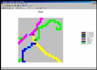
Slowly
move the cursor over the map and observe the map values associated with various
locations. The color levels identified
in the map legend aggregate the elevation values into ten 200-foot contour
intervals ranging from 500 to 2500.
![]() Click on the Layer mesh button on the
main tool bar. The grid configuration
for the Tutor25 database is 25 columns by 25 rows (25 x 25= 625 grid
cells). Each cell is 100 x 100 meters
(10,000 square meters; one hectare).
Several of the maps in the database are hypothetical and the Latitude
and Longitude coordinates for the project area were arbitrarily assigned. The contour lines and interactive data labels
for the Elevation map are interpolated “on-the-fly” from the underlying grid
data.
Click on the Layer mesh button on the
main tool bar. The grid configuration
for the Tutor25 database is 25 columns by 25 rows (25 x 25= 625 grid
cells). Each cell is 100 x 100 meters
(10,000 square meters; one hectare).
Several of the maps in the database are hypothetical and the Latitude
and Longitude coordinates for the project area were arbitrarily assigned. The contour lines and interactive data labels
for the Elevation map are interpolated “on-the-fly” from the underlying grid
data.
![]() Click on the Use cells button. The display switches from “lattice” to “grid”
display type with the contour color codes are assigned to entire cells. The important differences between lattice and
grid display types are covered in more detail in the MapCalc Application example entitled “Display Type.”
Click on the Use cells button. The display switches from “lattice” to “grid”
display type with the contour color codes are assigned to entire cells. The important differences between lattice and
grid display types are covered in more detail in the MapCalc Application example entitled “Display Type.”
![]() Click on the Toggle 3D view button. The display switches to a 3-D display in grid
cell display. The color-coding at the
top of each projected cell identifies its elevation.
Click on the Toggle 3D view button. The display switches to a 3-D display in grid
cell display. The color-coding at the
top of each projected cell identifies its elevation.
![]() The navigation tools enable you to zoom, pan
and rotate a display.
The navigation tools enable you to zoom, pan
and rotate a display.
ü
Click on the Zoom in button then click-and-drag
a rectangular portion of the displayed map to enlarge that area.
ü
Click on the Zoom out button then
click-and-hold while sliding up and down to continuously rescale the display
when you release the mouse button.
ü
Click on the Move button and click-and-hold to
move the display to another part of the screen.
ü
Click on the Rotate button and click-and-hold
as you rotate the plot cube.
ü
Click on the Reset view button to return to the
default display settings.
![]() Click off the Use cells button to
switch to a 3-D lattice display type, commonly called a “wireframe”
display. Note that the navigation tools
operate in the same manner for both the grid and lattice display types.
Click off the Use cells button to
switch to a 3-D lattice display type, commonly called a “wireframe”
display. Note that the navigation tools
operate in the same manner for both the grid and lattice display types.
![]() Click off and on the Layer contoured
and Layer contour lines buttons to turn off and on the contour-fill
colors and lines.
Click off and on the Layer contoured
and Layer contour lines buttons to turn off and on the contour-fill
colors and lines.
![]() Click off and on the Floor contours/lines
and Ceiling contours/lines buttons and note the changes in the 2-D
projected planes in the plot cube.
Click off and on the Floor contours/lines
and Ceiling contours/lines buttons and note the changes in the 2-D
projected planes in the plot cube.
Click
on the word “Map” in the main menu, then select “Overlay” and
choose the “Slope” map. The
result is a graphical overlay of the Slope map on the 3-D display of the
Elevation map. Note that the areas
classified as steep (green tones) align with the steepest portions of the
terrain surface.
![]() Click on the Arrange windows buttons
to view all of the open map windows in different arrangements. Click on the Maximize button in the
Slope map’s window to enlarge the display to fit the entire work area. For review, repeat the display tools
exercises you just completed using the elevation map on the Slope map.
Click on the Arrange windows buttons
to view all of the open map windows in different arrangements. Click on the Maximize button in the
Slope map’s window to enlarge the display to fit the entire work area. For review, repeat the display tools
exercises you just completed using the elevation map on the Slope map.
Clicking
on the word “Window” on the main menu produces a listing of open windows
and window management tools. Clicking on
any of the open map windows listed will cause that map to be maximized in the
work area.
![]() Click on the View, Rename and Delete
layers button to pop-up a listing of the current maps in the Tutor25
database. You can Rename and Delete
existing maps. As new maps are created
they are added to the list. The View
function opens a map in a new window. It
is important to note that you can have multiple windows open of the same
map. While this can cause some initial
confusion, experienced MapCalc users
find it useful for positioning side-by-side views of the same data, such as a
2-D display and a 3-D plot.
Click on the View, Rename and Delete
layers button to pop-up a listing of the current maps in the Tutor25
database. You can Rename and Delete
existing maps. As new maps are created
they are added to the list. The View
function opens a map in a new window. It
is important to note that you can have multiple windows open of the same
map. While this can cause some initial
confusion, experienced MapCalc users
find it useful for positioning side-by-side views of the same data, such as a
2-D display and a 3-D plot.
Exit
the Tutor25 database as described in “Exiting MapCalc” at the beginning of this Tutorial… do not save your
changes.
Lesson 2 – Understanding Data Types
Access
the Tutor25 database as described in “Starting MapCalc” at the beginning of this Tutorial.
The
Elevation map contains Continuous mapped data—the map values form a
gradient that changes throughout the map area.
The display tools described in Lesson 1 form appropriate plots of this
data type. In generating the displays a
numerical relationship is assumed to exist between the map values. For example, a the elevation of location that
is 2000 feet is twice as high as one that is 1000 feet. Similarly, a slope of 10 percent is much more
gentle than one of 30 percent.
However,
not all maps contain values that are numerically related. Discrete mapped data uses map values
simply to identify separate categories. For
example, a map of Roads might use the value 1 to denote backcountry roads and
the value 4 to identify highways.
Similarly, maps for administrative Districts might simply number
different districts or assign a numerical code.
 Click on the word “Window”
on the main menu and select the Roads map.
Click on the word “Window”
on the main menu and select the Roads map.
A
grid representation of a road map identifies the cells that contain a
road. In this example, the value zero is
assigned to all locations without a road.
Numbers are assigned to areas with roads in a manner that identifies the
type of road. Note that values 1-4 are
used for roads with increasingly greater traffic, value 5 is used for bridges,
and two-digit values form a code of the road types at each intersection. Clearly the map values do not represent
Continuous data and cannot be interpreted in the normal way—a road type 4 isn’t
four times bigger or better than a road type 1 (just different).
The
display of the Road map is as a Discrete Data type and provides the most
appropriate view of this kind of information.
![]() Click on the Layer mesh button on the
main tool bar. Move the cursor
throughout out the map and note the map categories corresponding to the
color-coding within the grid cells.
Click on the Layer mesh button on the
main tool bar. Move the cursor
throughout out the map and note the map categories corresponding to the
color-coding within the grid cells.
![]() Click on the Toggle 3D view button to
generate a 3-D view of the data. While
this view isn’t wrong, per se, it is inappropriate. In this view, the map values are considered
related and the two-digit codes for the intersections tower over the smaller
map values representing road type.
Click on the Toggle 3D view button to
generate a 3-D view of the data. While
this view isn’t wrong, per se, it is inappropriate. In this view, the map values are considered
related and the two-digit codes for the intersections tower over the smaller
map values representing road type.
![]() Click off the Use cells button to
switch to a 3-D lattice format. The
effect is similar to the 3-D grid type display and is just as
inappropriate.
Click off the Use cells button to
switch to a 3-D lattice format. The
effect is similar to the 3-D grid type display and is just as
inappropriate.
![]() Click off the Toggle 3D view button to
generate a 2-D view of the data. This
view of the data is as confusing as it is inappropriate because the display
attempts to establish color intervals between adjacent cells with different
values.
Click off the Toggle 3D view button to
generate a 2-D view of the data. This
view of the data is as confusing as it is inappropriate because the display
attempts to establish color intervals between adjacent cells with different
values.
![]() Click on the Data type button to
switch from Discrete data to Continuous data representation. Note, for the first time, the map values
appearing in the legend have changed.
This view treats the data range (minimum= 1 to maximum= 43) as number
gradient and divides the range into contour intervals. As depicted in the legend, red is assigned to
map values within the range 0 to 6.1—from no road to all road types and
bridges. The “bull’s-eye” looking
locations correspond to the two-digit intersections. This view is inappropriate and confusing as
well.
Click on the Data type button to
switch from Discrete data to Continuous data representation. Note, for the first time, the map values
appearing in the legend have changed.
This view treats the data range (minimum= 1 to maximum= 43) as number
gradient and divides the range into contour intervals. As depicted in the legend, red is assigned to
map values within the range 0 to 6.1—from no road to all road types and
bridges. The “bull’s-eye” looking
locations correspond to the two-digit intersections. This view is inappropriate and confusing as
well.
![]() Click on the Use cells button to
switch from lattice back to grid format.
The color-coding of this legend is still inappropriate as it treats the
data as continuous.
Click on the Use cells button to
switch from lattice back to grid format.
The color-coding of this legend is still inappropriate as it treats the
data as continuous.
![]() Click on the Data type button to
switch back to discrete data representation.
This display (2-D grid display type in Discrete data
format) is the only appropriate display for this type of data.
Click on the Data type button to
switch back to discrete data representation.
This display (2-D grid display type in Discrete data
format) is the only appropriate display for this type of data.
![]() Click on the Shading Manager button to
access the color pallet and labels for the Roads map. Click in the Category column next to
the value “0” and enter “No Road” as the label for that value. Change the color for that value by clicking
on the color and selecting another one from the basic color panels or by
clicking anywhere in the color gradient and pressing the OK button. Repeat labeling and color selection for other
map values. In the Shading manager
dialog box click the Apply button to store your label and color
assignments.
Click on the Shading Manager button to
access the color pallet and labels for the Roads map. Click in the Category column next to
the value “0” and enter “No Road” as the label for that value. Change the color for that value by clicking
on the color and selecting another one from the basic color panels or by
clicking anywhere in the color gradient and pressing the OK button. Repeat labeling and color selection for other
map values. In the Shading manager
dialog box click the Apply button to store your label and color
assignments.
For
review, click on the word “Window” on the main menu and select the
Districts map to display another example of a map containing discrete
data. Use the display tools to view the
map under different views as you did for the Roads map. Use the shading manager to recolor and label
the map.
Exit
the Tutor25 database as described in “Exiting MapCalc” at the beginning of this Tutorial… do not save your
changes.
Lesson 3 – Using the Shading Manager
Access
the Tutor25 database as described in “Starting MapCalc” at the beginning of this Tutorial.
![]() Click on the Shading Manager button to
access the color pallet and labels for the Elevation map. Another way to access the shading manager is
by right clicking anywhere within the map and selecting the Shading Manager
option.
Click on the Shading Manager button to
access the color pallet and labels for the Elevation map. Another way to access the shading manager is
by right clicking anywhere within the map and selecting the Shading Manager
option.
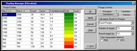 The shading manager for
continuous data contains two sections.
The left side interacts with the contour intervals and colors
assigned. The right side provides map
summaries and procedures for setting the display intervals. The button at the bottom toggles on (“More”)
and off (“Less”) the right side of shading manager dialog box.
The shading manager for
continuous data contains two sections.
The left side interacts with the contour intervals and colors
assigned. The right side provides map
summaries and procedures for setting the display intervals. The button at the bottom toggles on (“More”)
and off (“Less”) the right side of shading manager dialog box.
Color
assignments are changed by clicking on the color and selecting another from the
basic color panels or by clicking anywhere in the color gradient and pressing
the OK button. Change the color
assignments of the Elevation map by clicking on red (bottom), changing it to
blue and pressing OK. Repeat the process
to change green (top) to red. Note the
automatic assignment of other colors to the new color gradient. Press the Apply button to submit the
changes and generate a new display.
You
can set “Inflection points” within the color gradient. In this example, yellow is locked “On” and
effectively breaks the blue to red gradient into two gradients—blue to yellow
and yellow to red. Remove the yellow
inflection point by clicking on the word “On” (switches to “Off”). Press the Apply button to view the
change in the map. On your own, set the
yellow inflection point as the forth position from the top.
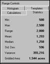 Click on the Statistics tab to get a
statistical summary of the map values.
Click on the Statistics tab to get a
statistical summary of the map values.
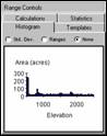 Click on the Histogram tab to get a
plot of the distribution of the map values.
Click on the Histogram tab to get a
plot of the distribution of the map values.
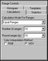 Click on the Calculations tab to activate the
interface for changing the display intervals.
There are two primary specifications needed to set the ranges used in
defining the intervals— 1) Number of Ranges and 2) Calculation Mode for Ranges.
Click on the Calculations tab to activate the
interface for changing the display intervals.
There are two primary specifications needed to set the ranges used in
defining the intervals— 1) Number of Ranges and 2) Calculation Mode for Ranges.
![]() Change the number of intervals from 10 to
5. Note the change in the upper and
lower values defining each of the five intervals and the number of grid cells
they contain. Press the Apply
button to view the map with the new interval assignments.
Change the number of intervals from 10 to
5. Note the change in the upper and
lower values defining each of the five intervals and the number of grid cells
they contain. Press the Apply
button to view the map with the new interval assignments.
![]() Use the drop down scroll list (down arrow
next to the “Calculation…” input field).
Change the “Equal Ranges” mode to Equal Count. Note the change in the upper and lower
values defining the intervals (right side) and the number of grid cells assigned
to each. Press the Apply button
to view the change in the map.
Use the drop down scroll list (down arrow
next to the “Calculation…” input field).
Change the “Equal Ranges” mode to Equal Count. Note the change in the upper and lower
values defining the intervals (right side) and the number of grid cells assigned
to each. Press the Apply button
to view the change in the map.
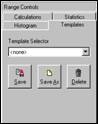 Click on the Template tab to store the
new display settings. Press the Save
As button and enter “Tutorial” as the name for the new display
template. Press the drop down scroll
list and retrieve any of the other current templates to apply to the map. Repeat to retrieve and reapply your
“Tutorial” template.
Click on the Template tab to store the
new display settings. Press the Save
As button and enter “Tutorial” as the name for the new display
template. Press the drop down scroll
list and retrieve any of the other current templates to apply to the map. Repeat to retrieve and reapply your
“Tutorial” template.
See
the MapCalc User Manual for more information on the considerations and
effects of interval calculations.
Exit
the Tutor25 database as described in “Exiting MapCalc” at the beginning of this Tutorial… do not save your
changes.
Lesson 4 – Setting Map Properties
Access
the Tutor25 database as described in “Starting MapCalc” at the beginning of this Tutorial.
Right-click
anywhere within the map and select the Properties option. Another way to access the dialog box is to
click on the word “Map” on the main menu and select “Properties.”
 Click on the Display tab to show the
basic settings for the current map display.
The buttons at the bottom enable you to apply the settings to all of the
other maps and/or store them as the default settings (global settings)—rarely
done. If you make changes in the
settings you can apply the changes to the current map by pressing the Apply
button at the bottom (individual map settings).
Click on the Display tab to show the
basic settings for the current map display.
The buttons at the bottom enable you to apply the settings to all of the
other maps and/or store them as the default settings (global settings)—rarely
done. If you make changes in the
settings you can apply the changes to the current map by pressing the Apply
button at the bottom (individual map settings).
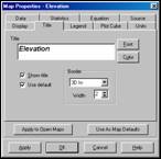 Click on the Title tab. This dialog box allows you to change the
title of the map and its appearance to include font type, font color, and
border characteristics. Use the Show
title checkbox to turn on and off the title in the map display. The Use default checkbox uses the map
name as the default title. If you want
to change the title click off the “Use default” checkbox, highlight the current
title and enter a new one.
Click on the Title tab. This dialog box allows you to change the
title of the map and its appearance to include font type, font color, and
border characteristics. Use the Show
title checkbox to turn on and off the title in the map display. The Use default checkbox uses the map
name as the default title. If you want
to change the title click off the “Use default” checkbox, highlight the current
title and enter a new one.
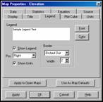 Click on the Legend tab to change the
map legend, its font and/or its appearance.
The Pos input filed enables you to position the legend at the
right, left, top or bottom of the work area.
Click on the Legend tab to change the
map legend, its font and/or its appearance.
The Pos input filed enables you to position the legend at the
right, left, top or bottom of the work area.
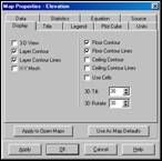
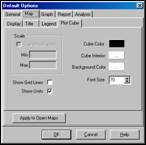
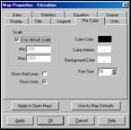 The Plot Cube tab enables you to
customize the appearance of the reference plot that appears in 3-D
displays. By far the most important
option involves the setting the Scale of the three-dimensional
plot. The Use default scale
checkbox automatically sets the minimum and maximum values for the Z-axis that produces
a pleasing vertical sizing of the map.
To manually set the min/max, click off the check box and enter –2000 as
the min and 4000 as the max then click the Apply button. Note that the plot has considerably less
vertical exaggeration. To eliminate the
plot cube click on Cube Color and change the color to white (background color).
The Plot Cube tab enables you to
customize the appearance of the reference plot that appears in 3-D
displays. By far the most important
option involves the setting the Scale of the three-dimensional
plot. The Use default scale
checkbox automatically sets the minimum and maximum values for the Z-axis that produces
a pleasing vertical sizing of the map.
To manually set the min/max, click off the check box and enter –2000 as
the min and 4000 as the max then click the Apply button. Note that the plot has considerably less
vertical exaggeration. To eliminate the
plot cube click on Cube Color and change the color to white (background color).
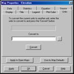 Click on the Units tab. Currently there are no units associated with
the Elevation map. To set map units
enter “feet”, press the Convert button (respond “yes” to use a
conversion factor of 1) and press the Apply button. Note that the units “feet” are now associated
with the map and are included in the map legend.
Click on the Units tab. Currently there are no units associated with
the Elevation map. To set map units
enter “feet”, press the Convert button (respond “yes” to use a
conversion factor of 1) and press the Apply button. Note that the units “feet” are now associated
with the map and are included in the map legend.
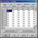 Click on the Data tab to view the map
values in table form. Use the slider
bars to scroll the columns (1 to 25 from left to right—X-axis with east at
right) and rows (1 to 25 from bottom to top—Y-axis with North at top). The next lesson will describe several other
procedures for data inspection and charting.
Click on the Data tab to view the map
values in table form. Use the slider
bars to scroll the columns (1 to 25 from left to right—X-axis with east at
right) and rows (1 to 25 from bottom to top—Y-axis with North at top). The next lesson will describe several other
procedures for data inspection and charting.
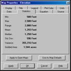 Click on the Statistics tab for a
listing of statistics summarizing the map values.
Click on the Statistics tab for a
listing of statistics summarizing the map values.
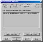 Click on the Equation tab for
information about how the map was created.
In this example, the Elevation map was imported form a data file in
Surfer format. Each map created by a MapCalc operation contains the complete
specification that derived it—metadata tracking.
Click on the Equation tab for
information about how the map was created.
In this example, the Elevation map was imported form a data file in
Surfer format. Each map created by a MapCalc operation contains the complete
specification that derived it—metadata tracking.
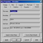 Click on the Source tab for
information about the database configuration.
Click on the Source tab for
information about the database configuration.
 Click on the word View on the main
menu then select “Options” to access the global default dialog box that allows
you to customize the “look-and-feel” of the software. Refer to the MapCalc User Manual for the procedures and settings available in
the Options dialog box.
Click on the word View on the main
menu then select “Options” to access the global default dialog box that allows
you to customize the “look-and-feel” of the software. Refer to the MapCalc User Manual for the procedures and settings available in
the Options dialog box.
Exit
the Tutor25 database as described in “Exiting MapCalc” at the beginning of this Tutorial… do not save your
changes.
Lesson 5 – Data Inspection and Charting
Access
the Tutor25 database as described in “Starting MapCalc” at the beginning of this Tutorial.
Recall
that the display type (lattice and grid) and data type (continuous
and discrete) greatly affects map display (see Lesson 2). Keep in mind, however that while the display
might change the underlying data stored in the map table is not changed.
By
slowly moving the cursor over a map a tracking window continuously updates the
value for each location. Maps containing
Continuous data report “display values” interpolated from the surrounding
“actual values” stored in the MapCalc
table. Discrete data maps report the
“category label” for the locations.
Click
on the word View on the main menu then select Data Inspection
option. A listing of all of the maps in
the database pops-up and is continuously updated for the actual data values as
the cursor is moved over the map. This
“drill-down” feature works for both 2-D and 3-D displays.
Click
on the words Map Set on the main menu, then select “New graph” and
choose “Histogram” to generate a plot of the data distribution of a map. Select the Slope map for a plot of its
data. Note that the scroll list only
shows maps that contain Continuous data.
Click
on the words Map Set on the main menu then select “New graph” and choose
“Scatterplot” to generate a plot of the joint frequency for a pair of
maps. Select the Slope map for the
X-axis and the Elevation map for the Y-axis.
The plot contains the regression line that graphically shows the
relationship between the two sets of mapped data. The regression equation and its R-squared
statistic indicating the strength of the relationship between the two maps
appear at the bottom of the plot.
![]() Click on the Print button to access
the report printing dialog box. Select
the Elevation map and press the button with a single arrow to move it to the
selected list box. Press the Preview
button for a mock-up of the printed page.
See the MapCalc User
Manual for more information on printing from MapCalc.
Click on the Print button to access
the report printing dialog box. Select
the Elevation map and press the button with a single arrow to move it to the
selected list box. Press the Preview
button for a mock-up of the printed page.
See the MapCalc User
Manual for more information on printing from MapCalc.
![]() Click on the Save picture button to
save a “screen grab” a basic image of the current map display. Any screen capture software, such as SnagIt
by Techsmith, can be used for more control on the type, position and
characteristics of the image.
Click on the Save picture button to
save a “screen grab” a basic image of the current map display. Any screen capture software, such as SnagIt
by Techsmith, can be used for more control on the type, position and
characteristics of the image.
Exit
the Tutor25 database as described in “Exiting MapCalc” at the beginning of this Tutorial… do not save your
changes.
Lesson 6 –Creating New Maps
Access
the Tutor25 database as described in “Starting MapCalc” at the beginning of this Tutorial.
![]() Click on the Map analysis button to
access the dialog box for creating new maps from existing mapped data by
applying MapCalc’s comprehensive set
of spatial statistics, analysis and modeling tools. This lesson covers the basic procedures for
specifying individual analysis operations and creating map analysis
macros. The online MapCalc
Applications document provides numerous examples of applying the complete
set of map analysis tools. In addition,
the online MapCalc User’s Manual contains more information about
features and capabilities of each analysis operation.
Click on the Map analysis button to
access the dialog box for creating new maps from existing mapped data by
applying MapCalc’s comprehensive set
of spatial statistics, analysis and modeling tools. This lesson covers the basic procedures for
specifying individual analysis operations and creating map analysis
macros. The online MapCalc
Applications document provides numerous examples of applying the complete
set of map analysis tools. In addition,
the online MapCalc User’s Manual contains more information about
features and capabilities of each analysis operation.
![]() Click on the Distance button and
select the “Spread” analysis operation.
Press the Help button to get information about the function and
specifications for Spread. Note that the
operation is used to “create a map indicating the shortest effective distance
from specified cells to all other locations.”
In this example, you will create a map that shows the distance from all
map locations to the nearest road location—proximity to roads.
Click on the Distance button and
select the “Spread” analysis operation.
Press the Help button to get information about the function and
specifications for Spread. Note that the
operation is used to “create a map indicating the shortest effective distance
from specified cells to all other locations.”
In this example, you will create a map that shows the distance from all
map locations to the nearest road location—proximity to roads.
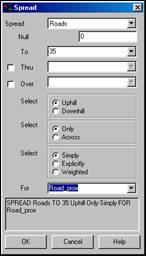 SPREAD Roads TO 35 Uphill Only Simply FOR
Road_prox
SPREAD Roads TO 35 Uphill Only Simply FOR
Road_prox
Complete
the specifications shown above by…
ü Spread <choose Roads> …as the map to measure distance
from
ü To <specify 35> …as the maximum
number of grid cells away from the roads
ü For <enter Road_prox> …as the name of the new map
created
ü …use the defaults for all of
the other options
Press
the OK button to create the proximity map.
Close the Map Analysis dialog box to view the Road_prox map—increasing
map values indicate areas farther away from roads. The farthest location is in the upper left
corner and is 10.7 cells away (10.7 cells * 100 m/cell = 1070 meters).
Click
on the word Windows on the main menu and select the Elevation map to
redisplay the map. Click on the word Map
then select “Overlay” and choose the “Road_prox” map you just created. In this display the information about
proximity to roads is graphically overlaid on the 3-D plot of the Elevation
surface.
![]() Click on the Map analysis button to
resurrect the analysis dialog box. Note
that your last entry is still there.
Double-click on the command line and the Spread operation’s dialog box
reappears. You can edit any
specification and rerun by clicking the OK button.
Click on the Map analysis button to
resurrect the analysis dialog box. Note
that your last entry is still there.
Double-click on the command line and the Spread operation’s dialog box
reappears. You can edit any
specification and rerun by clicking the OK button.
![]() Click on the Neighbors button and
select the “Slope” analysis operation.
Press the Help button to get information about the function and
specifications for Slope. Note that the
operation is used to “creates a map indicating the slope (1st derivative) along
a continuous surface.” In this example,
you will create a map that shows the terrain inclination for each map location
by fitting a plane to the nine elevation values surrounding the
location—terrain slope.
Click on the Neighbors button and
select the “Slope” analysis operation.
Press the Help button to get information about the function and
specifications for Slope. Note that the
operation is used to “creates a map indicating the slope (1st derivative) along
a continuous surface.” In this example,
you will create a map that shows the terrain inclination for each map location
by fitting a plane to the nine elevation values surrounding the
location—terrain slope.
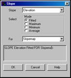 SLOPE Elevation Fitted FOR Slopemap
Complete
the specifications shown above by…
ü Slope <choose Elevation> …as the map to measure terrain
inclination
ü For <enter Slopemap> …as the name of the new map created
ü …use the defaults for all of
the other options
Press
the OK button to create a map of slope.
Close the Map Analysis dialog box to view the map—increasing map values
indicate steeper areas.
Click
on the word Windows on the main menu and select the “Elevation” map to
redisplay it. Click on the word Map
then select “Overlay” and choose the “Slopemap” you just created. In this display the information about terrain
slope is graphically overlaid on the 3-D plot of the Elevation surface.
Importing
and exporting grid data with other software packages is important. If you have the Surfer system installed
(bundled with MapCalc educational
version), you can automatically export, launch, and view maps in Surfer
software.
Right-click
anywhere on the “Elevation” map, then select “View in Surfer” and choose the
“Wireframe” display type. These
specifications launch a series of actions: the map is exported as a temporary
.GRD file; Surfer is activated; the .GRD file is imported; and a wireframe
display is generated. At this point the
Elevation map that originated in MapCalc
is fully available for Surfer processing.
Note that only the Elevation map (active map layer) was transferred
without the graphic overlay map of slope.
Direct
import/export in a variety of formats is supported provided the databases share
the same grid configuration. In this
example, you will import a map developed in Surfer software that shows the
level of animal activity.
![]()
![]() Click on the Map analysis button,
click on the Import/Export button and select “Import” to pop-up the
import dialog box.
Click on the Map analysis button,
click on the Import/Export button and select “Import” to pop-up the
import dialog box.
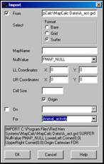 IMPORT C:\Program Files\Red Hen Systems\MapCalc\MapCalc Data\A_act.grd SURFER NullValue PMAP_NULL LowerLeft
Corner(0,0) UpperRight Corner(0,0) Origin Cartesian FOR Animal_activity
IMPORT C:\Program Files\Red Hen Systems\MapCalc\MapCalc Data\A_act.grd SURFER NullValue PMAP_NULL LowerLeft
Corner(0,0) UpperRight Corner(0,0) Origin Cartesian FOR Animal_activity
Complete
the specifications shown above by…
ü From <…A_activity.grd> …navigate to …\MapCalc\MapCalc
Data\A_activity.grd
ü Select <click Surfer> …identifies a Surfer .GRD
formatted file
ü For <enter Animal_activity> …as the name of the new map created
ü …use the defaults for all of
the other options
In
addition to direct import of grid data, MapCalc
creates map layers using columns of data you select from any *.tab (MapInfo
table format) or *.shp (ArcView
Exit
the Tutor25 database as described in “Exiting MapCalc” at the beginning of this Tutorial… do not save your
changes.
Taking the Next Step
The
lessons in this tutorial were designed to get you started. Some of the basic procedures for accessing,
displaying and creating maps were briefly introduced. Given this foundation you are ready for
further investigation MapCalc’s
capabilities.
Lesson
7 (below) is an example of a simple
The
MapCalc User Manual is another excellent place to continue your exposure
to MapCalc and the analytical capabilities of grid-based
processing. The first part of the manual
extends the tutorial experience through a detailed yet concise discussion of
setting program defaults, creating maps, working with maps and using the menus
and toolbars. The remaining part
provides description of the function and syntax for the map analysis
operations.
Once
you are comfortable with basic operation of MapCalc
you are ready to consider using it in solving spatial problems and constructing
As
your familiarity with MapCalc increases, you can input your own
data and begin developing your own spatial models—moving you beyond mapping
toward spatial reasoning and better information for decision-making.
Lesson 7 – GIS Modeling
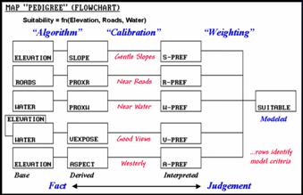 Situation

All
The
each row in the flowchart is evaluated to reflect preferences for locating a
campground—gentle slopes, near roads, near water, good views and westerly
oriented. The final step combines the
maps of the five criteria for a map of the overall suitability (SUITABLE).
Note
that the columns in the flowchart reflect increasing abstraction from Base
maps of physical features, to Derived maps of spatial context, to Interpreted
maps of relative goodness, and finally to a Modeled map of
suitability. The movement from maps of
physical Fact to decision Judgment involves a logical sequencing
of map analysis operations.
This
lesson provides hands-on experience in accessing and executing a command macro
that implements the campground location model described above.
Accessing a Stored Command Macro
Access
the Tutor25 database as described in “Starting MapCalc” at the beginning of this Tutorial.
Open
the command macro for the “Campground Suitability Model” by—
…access
the Grid Analysis module by pressing the Grid Analysis button on the
Main Toolbar
…select
Scriptà Open from the Map
Analysis menu
…navigate
to the C:\Program Files\Red Hen Systems\MapCalc\MapCalc Data\Scripts
folder
…open
the Campground.scr script
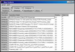 Command Macro Procedures

Each
line of the command macro contains an individual MapCalc command. The command lines are executed in their
listed order (top to bottom). You can
execute the entire command macro in “batch mode” by selecting Scriptà Run Script. You can view a command’s specifications by double-clicking
on a command line, then click “OK” to execute the command and display the
derived map.
Annotated Listing of Commands
note
...DEVELOPMENT MODEL -- fn(Elevation, Roads, Water)
note The best areas for development are those that are gently sloped, near roads, near water, good views of water, westerly oriented, and not legally 'constrained'.
note
...there are four submodels:
note Section 1 -- Derived maps
note Section 2 -- Interpreted maps
note Section 3 -- Constraints map
note Section 4 -- Suitability map
===========================================================
note
...Section 1] Derived Maps
note ELEVATION --- slope ---> SLOPEMAP
note ROADS
--- spread ---> PROXIMITY_ROADS
note WATER
--- spread ---> PROXIMITY_WATER
note WATER | ELEVATION --- radiate ---> EXPOSURE_WATER
note ELEVATION --- orient ---> ASPECTMAP
note
...1a] Generate map of slope
SLOPE ELEVATION FOR SLOPEMAP
note
...1b] Generate map of proximity to roads
SPREAD ROADS TO 100 FOR PROXIMITY_ROADS
note
...1c] Generate map of proximity to water
SPREAD WATER TO 100 FOR PROXIMITY_WATER
note
...1d] Generate map of visual exposure to water
RADIATE WATER OVER ELEVATION COMPLETELY TO 100 FOR EXPOSURE_WATER
note
...1e] Generate map of aspect
ORIENT ELEVATION FOR ASPECTMAP
===========================================================
note
...Section 2] Interpreted Maps (10-Best....1-Worst)
note SLOPEMAP --- renumber ---> S_PREF
note
note
note VIEWS
--- renumber ---> V_PREF
note ASPECTMAP --- renumber ---> A_PREF
note
...a common preference scale is used for all of the interpreted maps—
note 0= Not Available , 1= Poor, …, 5= Marginal, 6=
Acceptable, 7= Good, 8= Very Good, 9= Excellent
note ...2a] Slope preference (like it gently sloped)
RENUMBER SLOPEMAP ASSIGN 9 TO 0 THRU 5 ASSIGN 8 TO 5 THRU 15 ASSIGN 5 TO 15 THRU 25 ASSIGN 3 TO 25 THRU 40 ASSIGN 1 TO 40 THRU 100 FOR S_PREF
note
...2b] Proximity to road preference (like it near roads)
RENUMBER PROXIMITY_ROADS ASSIGN 9 TO 0 ASSIGN 8 TO .001 THRU 1.5 ASSIGN 7 TO 1.5 THRU 3 ASSIGN 3 TO 3 THRU 6 ASSIGN 1 TO 6 THRU 11 FOR R_PREF
note
...2c] Proximity to water preference (like it near water)
RENUMBER PROXIMITY_WATER ASSIGN 9 TO 0 THRU 2 ASSIGN 7 TO 2 THRU 4 ASSIGN 4 TO 4 THRU 6 ASSIGN 1 TO 6 THRU 100 FOR W_PREF
note
...2d] View of water preference (like good views of water)
RENUMBER EXPOSURE_WATER ASSIGN 9 TO 80 THRU 150 ASSIGN 8 TO 30 THRU 80 ASSIGN 5 TO 10 THRU 30 ASSIGN 3 TO 6 THRU 10 ASSIGN 1 TO 0 THRU 6 FOR V_PREF
note
...2e] Westerly oriented preference (like it westerly oriented)
RENUMBER ASPECTMAP ASSIGN 9 TO 6 THRU 8 ASSIGN 7 TO 1 THRU 2 ASSIGN 3 TO 4 THRU 5 ASSIGN 1 TO 3 FOR A_PREF
===========================================================
note
...Section 3] Constraints 'Masking' Map
note SLOPEMAP --- renumber ---> NO_SLOPE
note PROXIMITY_WATER --- renumber
---> NO_
note NO_SLOPE | NO_
note
...a binary “masking map” is created where 0= Not Available and 1= OK to
Develop
note
...3a] Not over 50% slope
RENUMBER SLOPEMAP ASSIGN 1 TO 0 THRU 50 ASSIGN 0 TO 50 THRU 1000 FOR NO_SLOPE
note
...3b] Not within 100 meters
RENUMBER PROX -W ASSIGN 0 TO 0 THRU 1.4 ASSIGN 1 TO 1.4 THRU 100 FOR NO_PROX
note
...3c] Combine individual constraints
COMPUTE NO-SLOPE TIMES NO-PROX FOR
CONSTRAINTS
===========================================================
note
...Section 4] Development Suitability Map
note S_PREF --|
note R_PREF --|
note W_PREF --|-- average ---> POTENTIAL
note V_PREF --|
note A_PREF --|
note POTENTIAL | CONSTRAINTS -- compute times
---> POTENTIAL_MASKED
note
...4a] Total individual preferences for overall campground suitability
COMPUTE S_PREF
note
...4a] Average individual preferences for overall campground suitability
CALCULATE POTENTIAL_TOTAL / 5.0 FOR POTENTIAL_AVERAGE
note
...4c] Eliminate constrained areas
COMPUTE CONSTRAINTS TIMES POTENTIAL_AVERAGE FOR POTENTIAL_MASKED
===========================================================
note
... There are three types of modifications that can be made to
note WEIGHTING of interpreted maps (use
the “times” option in the Analyze command)
note PARAMETERIZATION of preference maps
(change the “assign” phrases in Renumber)
note STRUCTURAL additions to model logic
(add new criteria such as being “in or near Forests”)
note
... try expressing some of YOUR thoughts.