Beyond Mapping
|
Map
Analysis book with companion CD-ROM for hands-on exercises and further reading |
GIS Represents Spatial Patterns and Relationships — discusses
the important differences among discrete mapping , continuous map surfaces and
map analysis
Statistically Compare Discrete Maps — discusses
procedures for comparing discrete maps
Statistically Compare Continuous Map Surfaces — discusses
procedures for comparing continuous map surfaces
Geographic Software Removes Guesswork from Map
Similarity — discusses
basic considerations and procedures for generating similarity maps
Use Similarity to Identify Data Zones — describes
level-slicing for classifying areas into zones containing a specified data
pattern
Use Statistics to Map Data Clusters — discusses
clustering for partitioning an are into separate data groups
Spatial Data Mining “Down on the Farm” — discusses
process for moving from Whole-Field to Site-Specific management
Spatial Data Mining Allows Users to Predict Maps — describes the basic concepts and procedures for
deriving equations that can be used to derive prediction maps
Stratify Maps to Make Better Predictions — illustrates
a procedure for subdividing an area into smaller more homogenous groups prior
to generating prediction equations
Author’s
Notes: The figures in this topic use MapCalcTM
software. An educational CD with online
text, exercises and databases for “hands-on” experience in these and other
grid-based analysis procedures is available for US$21.95
plus shipping and handling (www.farmgis.com/products/software/mapcalc/
).
<Click
here> right-click to download a printer-friendly version of this topic
(.pdf).
(Back to the Table of Contents)
______________________________
(GeoWorld, April 1999, pg.
24-25)
Many
of the topics in this book have discussed the subtle (and often not so subtle)
differences between mapping and map analysis.
Traditionally, mapping identifies distinct map features, or spatial
objects, linked to aggregated tables that are visually interpreted for spatial
relationships. The thematic mapping and
geo-query capabilities of this approach enable users to “see through” the
complexity of spatial data and the barrage of associated tables.
Map analysis, on the other hand, slogs around in the complexity of geographic
space, treating it as a continuum of varying responses and utilizing map-ematical
computations to uncover spatial relationships. A major distinction between the two approaches
lies in the extension of the traditional map elements of points, lines and
areas to map surfaces—an old concept that has achieved practical reality with
the advent of digital maps.
Zones
and Surfaces
Map surfaces, also termed spatial gradients, often are characterized by
grid-based data structures. In forming a
surface, the traditional representation based on irregular polygons is replaced
by a highly resolved matrix of grid cells superimposed over an area (top
portion of figure 1).
Figure 1. Comparison of zone (polygon) and surface (grid) representations for a continuous variable.
The
representation of the data range for the two approaches is radically
different. Consider the alternatives for
characterizing phosphorous levels throughout a farmer’s field. One approach, termed zone management, uses
air photos and a farmer’s knowledge to subdivide the field into similar areas (gray levels depicted on the left side of
figure 1). Soil samples are randomly
collected in the areas and the average phosphorous level is assigned to each
zone. These, plus other soil data
gathered for each of the zones are used to develop a fertilization program for
the field.
An alternative approach, termed site-specific management, systematically samples
the field, then interpolates these data for a
continuous map surface of phosphorous levels (right side of figure 1). First, note the similarities between the two
representations—the generalized levels (data range) for the zones correspond
fairly well with the map surface levels (the darkest zone tends to align with
the highest levels, while the lightest zone contains the lowest levels).
Now consider the differences between the two representations. Note that the zone approach assumes a
constant level (horizontal plane) of phosphorous within each zone (Zone#1(dark gray)= 55, Zone#2= 46 and Zone#3(light
gray)= 42, whereas the surface shows a gradient of change across the field
varying from 22 to 140). Two important
pieces of information are lost in the zone approach—the extreme high/low values
and the geographic distribution of the variation. This “missing” information severely limits
the potential for spatial analysis of the zone data.*
Ok, you’re not a farmer, so what’s to worry?
If you think about it, the bulk of
Surface Modeling
There are two ways to establish map surfaces—continuous
sampling and spatial analysis of a dispersed set samples. By far the best way is to continuously sample
and directly assign an actual measurement(s) to each grid cell. Remote sensing data with a measurement for
each pixel is good example of this data type.
Figure 2. Geo-referenced map surfaces
provide information about the unique combinations of data values occurring
throughout an area.
However, map surfaces often are derived by
statistically estimating a value for each grid cell based on a set of scattered
measurements. For example, locations of
a bank’s home equity loan accounts can be geo-coded by their street
address. Like “push-pins” stuck into a
map on the wall, clusters of accounts form discernable patterns. An account density surface is easily
generated by successively stopping at each grid cell and counting the number of
accounts within 1/8th of a mile.
In a similar fashion, an account value surface is generated by summing
the account values within the radius.
These surfaces show the actual “pockets” (peaks and pits) of the bank’s
customers. By contrast, a zonal approach
would simply assign the average number/value of accounts “falling into”
predefined city neighborhoods, whether they actually matched the spatial
patterns in the data or not.
Surface
Analysis
The assumption of the zone approach is that the coincidence of the averages is
consistent throughout the entire map area.
If there is a lot of spatial dependency among the variables and the
zones happen to align with actual patterns in the data, this assumption isn’t
bad. However in reality this is rarely
the case.
Table 1. Comparison of zone and surface data for selected locations.
Consider the “shishkebab”
of data values for the four pins shown in Table 1. The first two pins are in Zone #1 so the
assumption is that the levels of phosphorous= 55, potassium= 457 and PH= 6.4
are the same for both locations (as they are for everywhere within Zone
#1). But the surface data for Pin #1
indicates a sizable difference from the averages—150% ([[140-55]/55]*100) for
phosphorous, 28% for potassium and 8% for PH.
The differences are less for Pin #2 with 20%, 2% and –2%,
respectively. Pins #3 and #4 are in
different zones, but similar deviations from the averages are noted, with the
greatest differences in phosphorous levels and the least in PH levels.
While zones might be sufficient for general description and viewing of
spatial data, surfaces are needed in most applications to discover spatial
relationships. As
________________
Author’s Note: a more detailed discussion
of zones and surfaces is available online at www.innovativegis.com/basis, select Column Supplements.
Statistically Compare
Discrete Maps
(GeoWorld, July 2006, pg. 16-17)
One of the most fundamental techniques in map analysis is the comparison of two maps. Questions like “…how different are they?”, “…how are they different?” and “…where are they different?” immediately spring to mind. Quantitative answers are needed because visual comparison cannot fully consider all of the spatial detail in an objective manner.
The two maps shown in figure 12-1 identify crop yield for successive seasons (1997 and 1998) on the central-pivot cornfield. Note that the maps have a common legend from 0 to 300 bushels per acre. How different are the maps? How are they different? And where are they different? While your eyes flit back and forth in an attempt to visually compare the maps, the computer approaches the problem much more methodically.
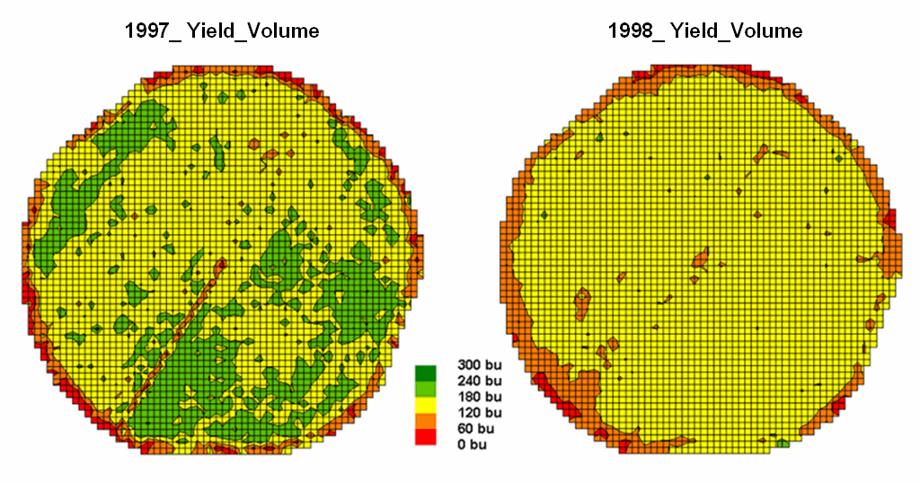
Figure 1. Discrete
yield maps for consecutive years.
In this Precision Agriculture application, thousands of
point values for yield are collected “on-the-fly” as a
The next step, as shown in figure 2, combines the two maps into a single map indicating the “joint condition” for both years. Since the two maps have an identical grid configuration, the computer simply retrieves the two class assignments for a grid location, and then converts them to a single number by computing the “first value times ten plus the second value” to form a two-digit code. In the example shown in the figure, the value “forty-three” is interpreted as class 4 in the first year but decreasing to class 3 in the next year.
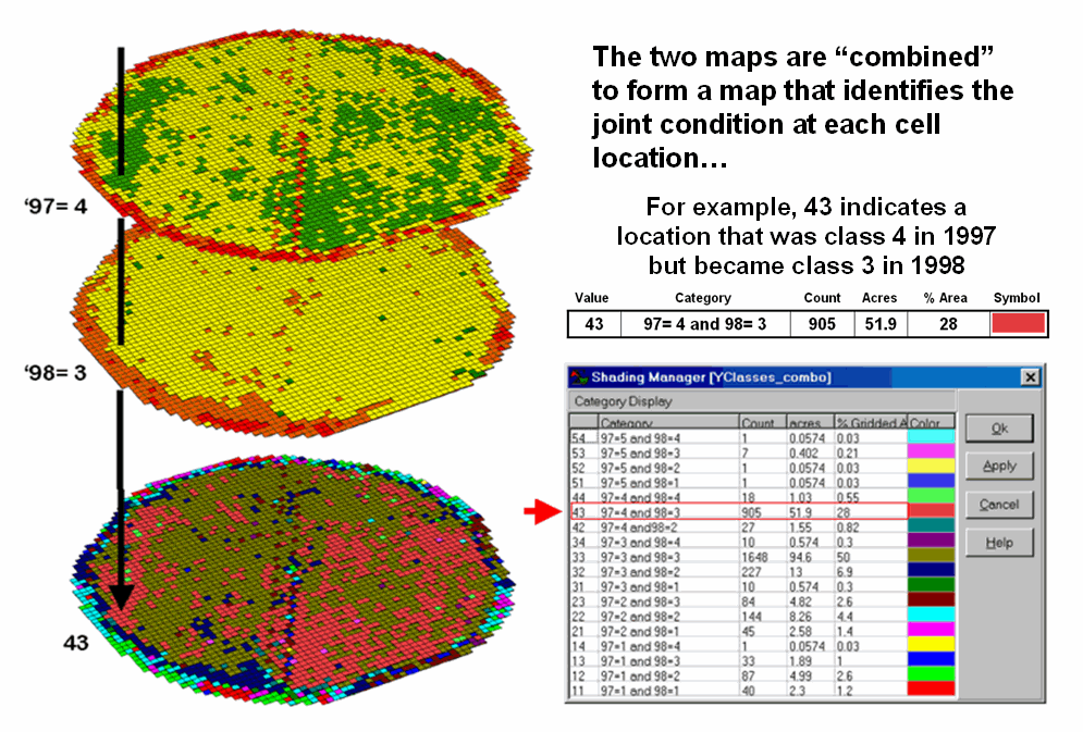
Figure 2. Coincidence
map identifying the joint conditions for both years.
The final step sums up the changes to generate the Coincidence Table shown in figure 3. The columns and rows in the table represent the class assignments on the 1997 and 1998 yield maps, respectively. The body of the table reports the number of cells for each joint condition. For example, column 4 and row 3 notes that there are 905 occurrences where the yield class slipped from level four (180-240bu/ac) to level three (120-180bu/ac).
The off-diagonal entries indicate changes between the two maps—the values indicate the relative importance of the change. For example, the 905 count for the “four-three” change is the largest and therefore identifies the most frequently occurring change in the field. The 0 statistic for the “four-one” combination indicates that level four never slipped all the way to level 1. Since the sum of the values above the diagonal (1224) is much larger than those below the diagonal (215), it clearly indicates that the downgrading of the yield classes dominates the change occurring in the field.
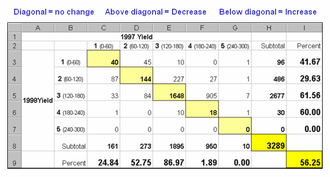
Figure 3. Coincidence summary table.
The diagonal entries summarize the agreement between the two maps. Generally speaking, the maps are very different as only a little more than half the field didn’t change (40+144+1648+18= 1850/3289= 56.25%). The greatest portion of the field that didn’t change occurs for yield class 3 (“three-three” with 1648 out of 1895 cells). The greatest difference occurred for class 4 (“four-four” with only 18/3289= 1.89% that didn’t change). The statistics in the table are simply summaries of the detailed spatial patterns of change depicted in the coincidence map shown in figure 2.
That’s a lot more meat in the answers to the basic map comparison questions (how much, how and where) than visceral viewing and eye flickering impression can do. Next month’s column focuses on even more precise procedures for quantifying differences using two continuous map surfaces.
Statistically Compare
Continuous Map Surfaces
(GeoWorld, September, 2006, pg. 24-25)
Contour maps are the most frequently used and familiar form of presenting precision agriculture data. The two 3D perspective-plots in the top of figure 1 show the color-coded ranges of yield (0-60, 60-120, etc. bushels per acre) and are identical to the discrete maps discussed in the previous section. The color-coding of the contours is draped for cross-reference onto the continuous 3D surface of the actual yield data.
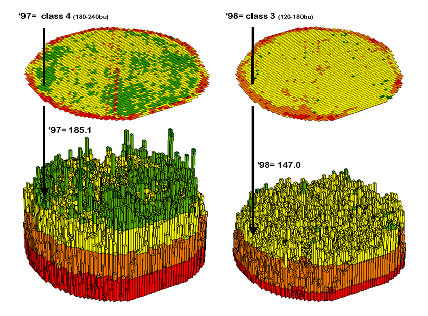
Figure 1. 3-D Views of yield surfaces for consecutive years.
Note the “spikes and pits” in the surfaces that graphically portray the variance in yield data for each of the contour intervals. While discrete map comparison identifies shifts in broadly defined yield classes, continuous surface comparison identifies the precise difference at each location.
For example, a yield
value of 179 bushels on one map and 121 on the other are both assigned to the
third contour interval (120 to180; yellow). A discrete map comparison would suggest that
no change in yield occurred for the location because the contour interval
remained constant. A continuous surface
comparison, would report a fairly significant 58-bushel decline.
Figure 2 shows the calculations using the actual values for the same location highlighted in the previous section’s discussion. The discrete map comparison reported a decline from yield level 4 (180 to 240) to level 3 (120 to 180).
The MapCalc command, “Compute Yield_98 minus Yield_97 for Difference” generates the difference surface. If the simple “map algebra” equation is expanded to “Compute (((Yield_98 minus Yield_97) / Yield_97) *100)” a percent difference surface would be generated. Keep in mind that a map surface is merely a spatially organized set of numbers that awaits detailed analysis then transformation to generalized displays and reports for human consumption.
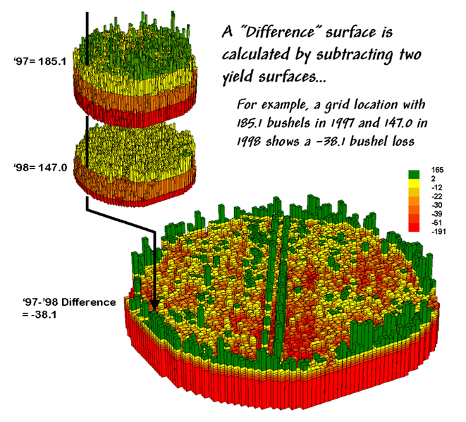
Figure 2. A
difference surface identifies the actual change in crop yield at each map
location.
In figure 2, note that the wildest differences (side-by-side green spikes and red pits) occur at the field edges and along the access road—from an increase of 165 bushels to a decrease of 191 bushels between the two harvests. However, notice that most of the change is about a 25 bushel decline (mean= -22.6; median= -26.3) as identified in the summary table shown in figure 12-6.
The continuous surface comparison more precisely reports the change as –38.1 bushels. The differences for other 3,289 grid cells are computed to derive a Difference Surface that tracks the subtle variations in the spatial pattern of the changes in yield.
The histogram of the yield differences in the figure shows the numerical distribution of the difference data. Note that it is normally distributed and that the bulk of the data is centered about a 25 bushel decline. The vertical lines in the histogram locate the contour intervals used in the 2D display of the difference map in the left portion of figure 3.
The detailed legend links the color-coding of the map intervals to some basic frequency statistics. The example location with the calculated decline of –38.1 is assigned to the –39 to –30 contour range and is displayed as a mid-range red tone. The display uses an Equal Count method with seven intervals, each representing approximately 15% of the field. Green is locked for the only interval of increased yield. The decreased yield intervals form a color-gradient from yellow to red. All in all, surface map comparison provides more information in a more effective manner discrete map comparison. Both approaches, however, are far superior to simply viewing a couple yield maps side-by-side and guessing at the magnitude and pattern of the changes.
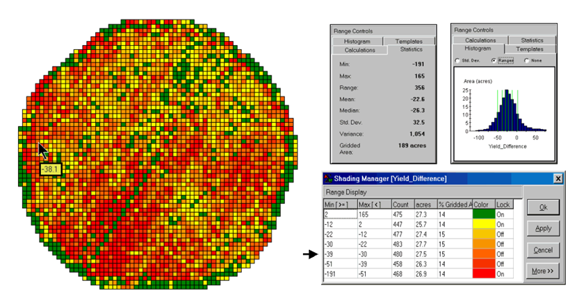
Figure 3. A 2-D map and
statistics summarize the differences in crop yield between two periods.
The ability to quantitatively evaluate continuous surfaces is fundamental to precision agriculture. A difference surface is one of the simplest and most intuitive forms. While the math and stat of other procedures are fairly basic, the initial thought of “you can’t do that to a map” is usually a reflection of our non-spatial statistics and paper-map legacies. In most instances, precision agriculture is simply an extension of current research and management practices from a few sample plots to extensive mapped data sets. The remainder of this case study investigates many of these extensions.
Geographic Software Removes Guesswork from
Map Similarity
(GeoWorld, October 2001, pg. 24-25)
How often have
you seen a
But just how similar is one location to another? Really similar, or just a little similar? And just how dissimilar are all of the other areas? While visceral analysis can identify broad relationships it takes a quantitative map analysis approach to handle the detailed scrutiny demanded in site-specific management.
Consider the three maps shown in figure 1— what areas identify similar patterns? If you focus your attention on a location in the southeastern portion how similar are all of the other locations?
The answers to these questions are much too complex for visual analysis and certainly beyond the geo-query and display procedures of standard desktop mapping packages. While the data in the example shows the relative amounts of phosphorous, potassium and nitrogen throughout a cornfield, it could as easily be demographic data representing income, education and property values. Or sales data tracking three different products. Or public health maps representing different disease incidences. Or crime statistics representing different types of felonies or misdemeanors.
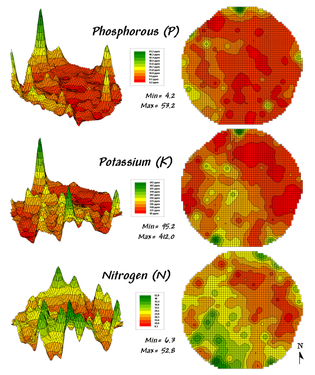
Figure 1. Map surfaces identifying the spatial
distribution of P,K and N
throughout a field.
Regardless of the data and application arena, the map-ematical procedure for assessing similarity is the same. In visual analysis you move your eye among the maps to summarize the color assignments at different locations. The difficulty in this approach is two-fold— remembering the color patterns and calculating the difference. The map analysis procedure does the same thing except it uses map values in place of the colors. In addition, the computer doesn’t tire as easily and completes the comparison for all of the locations throughout the map window (3289 in this example) in a couple seconds.
The upper-left portion of figure 2 illustrates capturing the data patterns of two locations for comparison. The “data spear” at map location 45column, 18row identifies that the P-level as 11.0ppm, the K-level as 177.0 and N-level as 32.9. This step is analogous to your eye noting a color pattern of burnt-red, dark-orange and light-green. The other location for comparison (32c, 62r) has a data pattern of P= 53.2, K= 412.0 and N= 27.9. Or as your eye sees it, a color pattern of dark-green, dark-green and yellow.
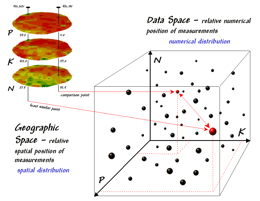
Figure 2. Conceptually linking geographic space and data space.
The right side of figure 2 conceptually depicts how the computer calculates a similarity value for the two response patterns. The realization that mapped data can be expressed in both geographic space and data space is key to understanding the procedure.
Geographic space uses coordinates, such latitude and longitude, to locate things in the real world—such as the southeast and extreme north points identified in the example. The geographic expression of the complete set of measurements depicts their spatial distribution in familiar map form.
Data space, on the other hand, is a bit less familiar. While you can’t stroll through data space you can conceptualize it as a box with a bunch of balls floating within it. In the example, the three axes defining the extent of the box correspond to the P, K and N levels measured in the field. The floating balls represent grid cells defining the geographic space—one for each grid cell. The coordinates locating the floating balls extend from the data axes—11.0, 177.0 and 32.9 for the comparison point. The other point has considerably higher values in P and K with slightly lower N (53.2, 412.0, 27.9) so it plots at a different location in data space.
The bottom line is that the position of any point in data space identifies its numerical pattern—low, low, low is in the back-left corner, while high, high, high is in the upper-right corner. Points that plot in data space close to each other are similar; those that plot farther away are less similar.
In the example, the floating ball closest to you is the farthest one (least similar) from the comparison point. This distance becomes the reference for “most different” and sets the bottom value of the similarity scale (0%). A point with an identical data pattern plots at exactly the same position in data space resulting in a data distance of 0 that equates to the highest similarity value (100%).
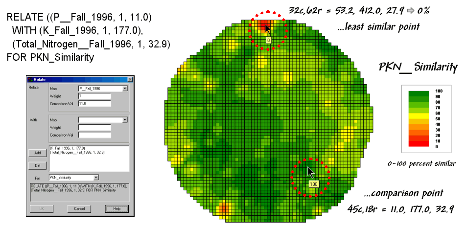
Figure 3. A
similarity map identifying how related locations are to a given point.
The similarity map shown in figure 3 applies the similarity scale to the data distances calculated between the comparison point and all of the other points in data space. The green tones indicate field locations with fairly similar P, K and N levels. The red tones indicate dissimilar areas. It is interesting to note that most of the very similar locations are in the western portion of the field.
A similarity map can be an invaluable tool for investigating spatial patterns in any complex set of mapped data. While humans are unable to conceptualize more than three variables (the data space box), a similarity index can handle any number of input maps. The different layers can be weighted to reflect relative importance in determining overall similarity.
In effect, a similarity map
replaces a lot of laser-pointer waving and subjective suggestions of
similar/dissimilar areas with a concrete, quantitative measurement at each map
location. The technique moves map analysis
well beyond the old “I’d never have seen, it if I hadn’t believe it” mode of
cartographic interpretation.
Use Similarity to Identify Data Zones
(GeoWorld,
November 2001, pg. 24-25)
The previous discussion introduced the concept of “data distance” as a means to measure similarity within a map. One simply mouse-clicks a location and all of the other locations are assigned a similarity value from 0 (zero percent similar) to 100 (identical) based on a set of specified maps. The statistic replaces difficult visual interpretation of map displays with an exact quantitative measure at each location.
An extension to the technique allows you to circle an area then compute similarity based on the typical data pattern within the delineated area. In this instance, the computer calculates the average value within the area for each map layer to establish the comparison data pattern, and then determines the normalized data distance for each map location. The result is a map showing how similar things are to the area of interest.
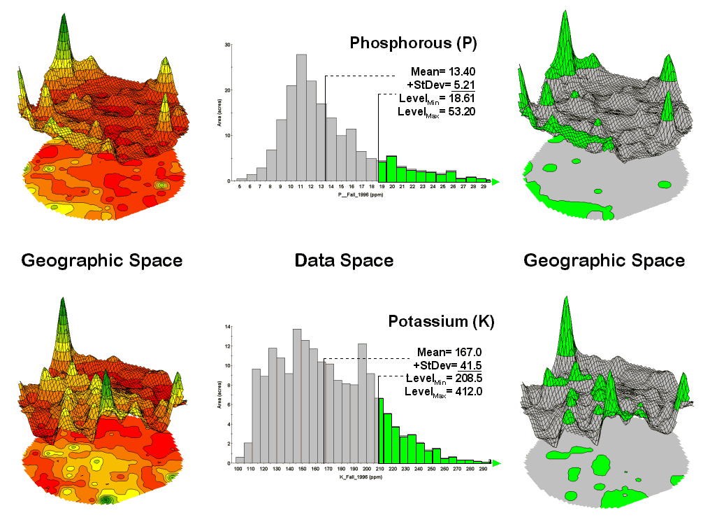
Figure 1. Identifying areas of
unusually high measurements.
In the same way, a marketer could use an existing sales map to identify areas of unusually high sales for a product, then generate a map of similarity based on demographic data. The result will identify locations with a similar demographic pattern elsewhere in the city. Or a forester might identify areas with similar terrain and soil conditions to those of a rare vegetation type to identify other areas to encourage regeneration.
The link between Geographic Space and Data Space is key. As shown in figure 1, spatial data can be viewed as a map or a histogram. While a map shows us “where is what,” a histogram summarizes “how often” measurements occur (regardless where they occur).
The top-left portion of the figure shows a 2D/3D map display of the relative amount of phosphorous (P) throughout a farmer’s field. Note the spikes of high measurements along the edge of the field, with a particularly big spike in the north portion.
The histogram to the right of the map view forms a different perspective of the data. Rather than positioning the measurements in geographic space it summarizes their relative frequency of occurrence in data space. The X-axis of the graph corresponds to the Z-axis of the map—amount of phosphorous. In this case, the spikes in the graph indicate measurements that occur more frequently. Note the high occurrence of phosphorous around 11ppm.
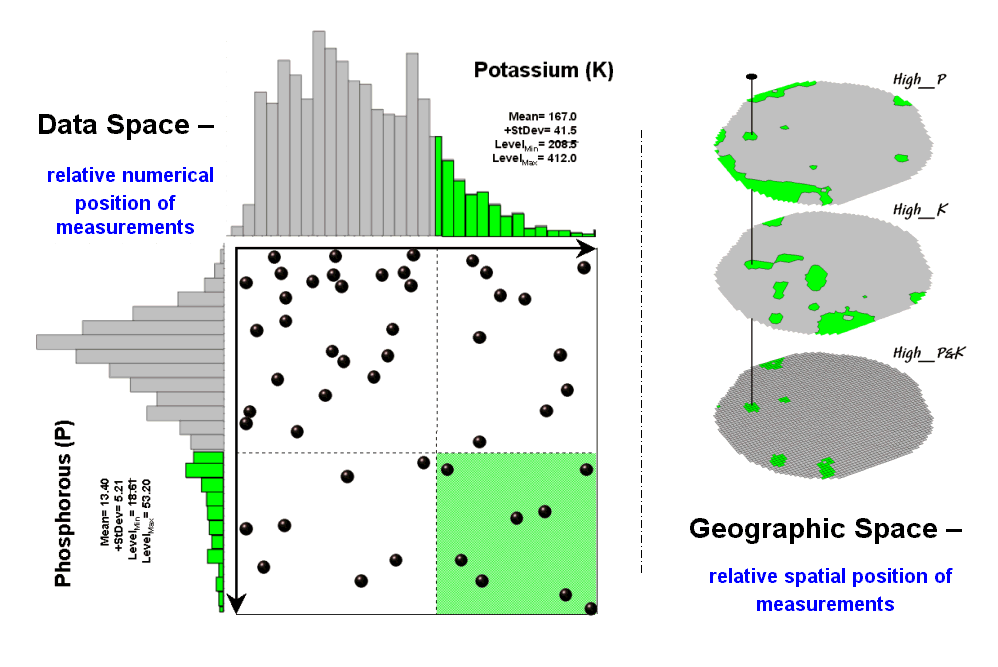
Figure 2. Identifying joint coincidence in both data and geographic space.
Now to put the geographic-data space link to use. The shaded area in the histogram view identifies measurements that are unusually high—more than one standard deviation above the mean. This statistical cutoff is used to isolate locations of high measurements as shown in the map on the right. The procedure is repeated for the potassium (K) map surface to identify its locations of unusually high measurements.
Figure 2 illustrates combining the P and K data to locate areas in the field that have high measurements in both. The graphic on the left is termed a scatter diagram or plot. It graphically summarizes the joint occurrence of both sets of mapped data.
Each ball in the scatter plot schematically represents a location in the field. Its position in the plot identifies the P and K measurements at that location. The balls plotting in the shaded area of the diagram identify field locations that have both high P and high K. The upper-left partition identifies joint conditions in which neither P nor K are high. The off-diagonal partitions in the scatter plot identify locations that are high in one but not the other.
The aligned maps on the right show the geographic solution for areas that are high in both of the soil nutrients. A simple map-ematical way to generate the solution is to assign 1 to all locations of high measurements in the P and K map layers (bight green). Zero is assigned to locations that aren’t high (light gray). When the two binary maps (0/1) are multiplied a zero on either map computes to zero. Locations that are high on both maps equate to 1 (1*1 = 1). In effect, this “level-slice” technique maps any data pattern you specify… just assign 1 to the data interval of interest for each map variable.
Figure 3 depicts level slicing for areas that are unusually high in P, K and N (nitrogen). In this instance the data pattern coincidence is a box in 3-dimensional scatter plot space.
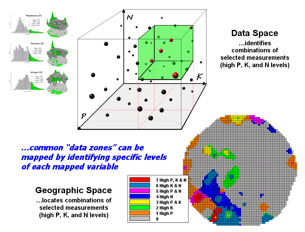
Figure 3. Level-slice classification using three map variables.
However a map-ematical trick was employed to get the map solution shown in the figure. On the individual maps, high areas were set to P=1, K= 2 and N=4, then the maps were added together.
The result is a range of coincidence values from zero (0+0+0= 0; gray= no high areas) to seven (1+2+4= 7; red= high P, high K, high N). The map values in between identify the map layers having high measurements. For example, the yellow areas with the value 3 have high P and K but not N (1+2+0= 3). If four or more maps are combined, the areas of interest are assigned increasing binary progression values (…8, 16, 32, etc)—the sum will always uniquely identify the combinations.
While level-slicing isn’t a very sophisticated classifier, it does illustrate the useful link between data space and geographic space. This fundamental concept forms the basis for most geostatistical analysis… including map clustering and regression to be tackled in the next couple of columns.
Use Statistics to Map
Data Clusters
(GeoWorld,
December 2001, pg. 24-25)
The last couple of sections have focused on analyzing data similarities within a stack of maps. The first technique, termed Map Similarity, generates a map showing how similar all other areas are to a selected location. A user simply clicks on an area and all other map locations are assigned a value from 0 (0% similar—as different as you can get) to 100 (100% similar—exactly the same data pattern).
The other technique, Level Slicing, enables a user to specify a data range of interest for each map in the stack then generates a map identifying the locations meeting the criteria. Level Slice output identifies combinations of the criteria met—from only one criterion (and which one it is), to those locations where all of the criteria are met.
While both of these techniques are useful in examining spatial relationships, they require the user to specify data analysis parameters. But what if you don’t know what Level Slice intervals to use or which locations in the field warrant Map Similarity investigation? Can the computer on its own identify groups of similar data? How would such a classification work? How well would it work?
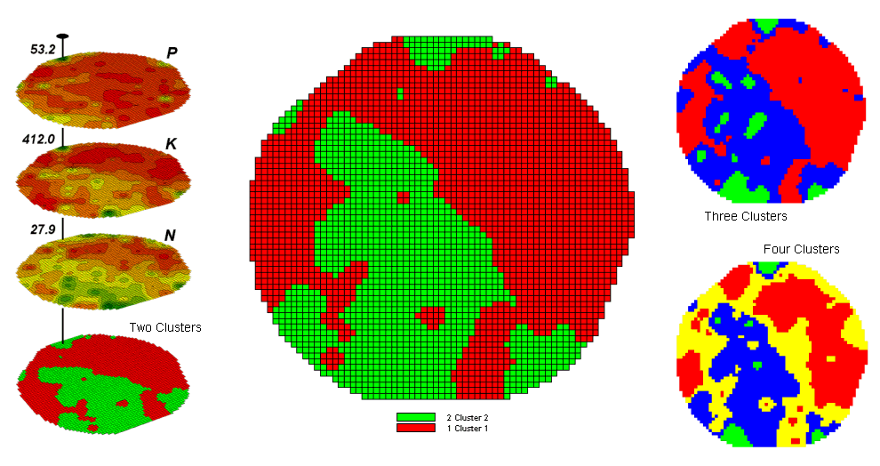
Figure 1. Examples of Map Clustering.
Figure 1 shows some examples derived from Map
Clustering. The “floating” maps on
the left show the input map stack used for the cluster analysis. The maps are the same P, K, and N maps
identifying phosphorous, potassium and nitrogen levels throughout a cornfield
that were used for the examples in the previous topics. However, keep in mind that the input maps
could be crime, pollution or sales data—any set of application related
data. Clustering simply looks at the
numerical pattern at each map location and ‘sorts” them into discrete groups.
The map in the center of the figure shows the results of classifying the P, K and N map stack into two clusters. The data pattern for each cell location is used to partition the field into two groups that are 1) as different as possible between groups and 2) as similar as possible within a group. If all went well, any other division of the field into two groups would be not as good at balancing the two criteria.
The two smaller maps at the right show the division of the data set into three and four clusters. In all three of the cluster maps red is assigned to the cluster with relatively low responses and green to the one with relatively high responses. Note the encroachment on these marginal groups by the added clusters that are formed by data patterns at the boundaries.
The mechanics of generating cluster maps are quite simple. Simply specify the input maps and the number of clusters you want then miraculously a map appears with discrete data groupings. So how is this miracle performed? What happens inside cluster’s black box?
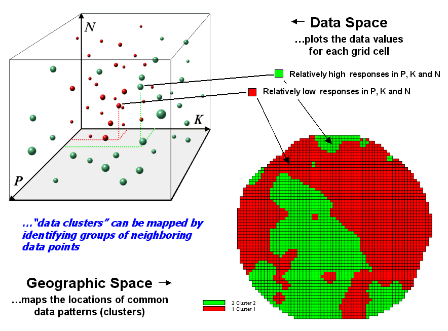
Figure 2.
Data patterns for map locations are depicted as floating balls in data
space.
The schematic in figure 2 depicts the process. The floating balls identify the data patterns for each map location (geographic space) plotted against the P, K and N axes (data space). For example, the large ball appearing closest to you depicts a location with high values on all three input maps. The tiny ball in the opposite corner (near the plot origin) depicts a map location with small map values. It seems sensible that these two extreme responses would belong to different data groupings.
The specific algorithm used in clustering was discussed in a previous Beyond Mapping column (see “Identifying Data Patterns,” Topic 7, Map Analysis). However for this discussion, it suffices to note that “data distances” between the floating balls are used to identify cluster membership—groups of balls that are relatively far from other groups and relatively close to each other form separate data clusters. In this example, the red balls identify relatively low responses while green ones have relatively high responses. The geographic pattern of the classification is shown in the map at the lower right of the figure.
Identifying groups of neighboring data points to form clusters can be tricky business. Ideally, the clusters will form distinct “clouds” in data space. But that rarely happens and the clustering technique has to enforce decision rules that slice a boundary between nearly identical responses. Also, extended techniques can be used to impose weighted boundaries based on data trends or expert knowledge. Treatment of categorical data and leveraging spatial autocorrelation are other considerations.
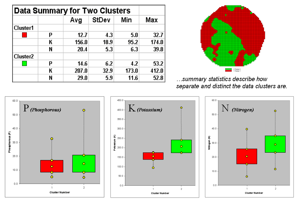
Figure 3. Clustering
results can be roughly evaluated using basic statistics.
So how do know if the clustering results are acceptable? Most statisticians would respond, “you can’t tell for sure.” While there are some elaborate procedures focusing on the cluster assignments at the boundaries, the most frequently used benchmarks use standard statistical indices.
Figure 3 shows the performance table and box-and-whisker plots for the map containing two clusters. The average, standard deviation, minimum and maximum values within each cluster are calculated. Ideally the averages would be radically different and the standard deviations small—large difference between groups and small differences within groups.
Box-and-whisker plots enable us to
visualize these differences. The box is
centered on the average (position) and extends above and below one standard
deviation (width) with the whiskers drawn to the minimum and maximum values to
provide a visual sense of the data range.
When the diagrams for the two clusters overlap, as they do for the
phosphorous responses, it tells us that the clusters aren’t very distinct along
this axis. The separation between the
boxes for the K and N axes suggests greater distinction between the clusters. Given the results a practical
Spatial Data Mining “Down
on the Farm”
(GeoWorld,
August 2006, pg. 20-21)
Until the 1990s, maps played a minor role in production agriculture. Most soil maps and topographic sheets were too generalized for use at the farm level. As a result, the principle of Whole-Field Management based on broad averages of field data, dominated management actions. Weigh-wagon and grain elevator measurements established a field's overall yield performance, and soil sampling determined the typical/average nutrient levels for a field. Farmers used such data to determine best overall seed varieties, fertilization rates and a bushel of other decisions that all treated an entire field as uniform within its boundaries.
Precision Agriculture, on the other hand, recognizes the variability within a field and involves doing the right thing, in the right way, at the right place and time—Site-Specific Management. The approach involves assessing and reacting to field variability by tailoring management actions, such as fertilization levels, seeding rates and selection variety, to match changing field conditions. It assumes that managing field variability leads to cost savings and production increases as well as improved stewardship and environmental benefits.
Figure 1 outlines the major steps in transforming spatial data and derived relationships into on-the-fly variable rate maps that puts a little here, more over there and none at other places in the field. The prescription maps are derived by applying spatial data mining techniques to uncover the relationship between crop production and management variables, such as fertility applications of phosphorous, potassium and nitrogen (P, K and N).
Figure 1. Relationships among yield and
field nutrient levels are analyzed to derive a prescription map that identifies
site-specific adjustments to nutrient application.
First a detailed map of crop yield is constructed by
on-the-fly yield monitoring as a harvester moves through a field. A record of the yield volume and
These data are analyzed to relate the spatial variations in
yield to the nutrient data patterns in the field (spatial
dependency/correlation) using such techniques as map comparison, similarity
analysis, zoning, clustering, regression and other statistical approaches (see
Author’s note). Once viable
relationships are identified, a prescription map is generated that instructs
on-the-fly application of varying nutrient inputs as a
Some might thing precision farming is an oxymoron when
reality is mud up to the axels and 400 acres to plow; however sophisticated
uses of geotechnology are rapidly changing production
agriculture. In just ten years it has become
nearly impossible to purchase equipment without wiring for
What really is revolutionary is the changing mindset from whole-field to site-specific management and the spatial data mining process used to derive spatial relationships that translate geographic variation in data patterns into prescription maps. Figure 2 depicts a generalized flowchart of the process that can be applied to a number of disciplinary fields.
Figure 2. A similar process for mining and utilizing spatial relationships can
be applied to other disciplinary fields.
For example, my first encounter with spatial data mining procedures was in extending a test market project for a phone company in the early 1990s. Customer addresses were used to geo-code map coordinates for sales of a new product enabling different rings to be assigned to a single phone line—one for the kids and another for the parents. Like pushpins on a map, the pattern of sales throughout the test market area emerged with some areas doing very well, while other areas sales were few and far between.
The demographic data for the city was analyzed to calculate
a prediction equation between product sale and census block data. The equation then was applied to another city
by evaluating existing demographics to “solve the equation” for a predicted
sales map. In turn, the predicted sales
map was combined with a wire-exchange map to identify switching faculties that
required upgrading before release of the product in the
Crop yield and sales yield at first might seem worlds apart, as do the soil nutrient and demographic variables that drive them. However from an analytical point of view the process is identical—just the variables are changed to protect the innocent. It leads one to wonder what other application opportunities await a paradigm shift from traditional to spatial statistics in other disciplines.
______________________________
Author’s Note: For more information on Precision Agriculture, see feature article
“Who’s Minding the Farm” (GeoWorld, February, 1998) or shortened online version
at www.geoplace.com/ge/2000/0800/0800pa.asp (GeoEurope).
Spatial Data Mining
Allows Users to Predict Maps
(GeoWorld,
January 2002, pg. 20-21)
Talk about the
future of
Extending
predictive analysis to mapped data seems logical. After all, maps are just organized sets of
numbers. And
If fact, the first time I used prediction mapping was in 1991 to extend a test market project for a phone company. The customer’s address was used to geo-code sales of a new product that enabled two numbers with distinctly different rings to be assigned to a single phone— one for the kids and one for the parents. Like pushpins on a map, the pattern of sales throughout the city emerged with some areas doing very well, while in other areas sales were few and far between.
The demographic
data for the city was analyzed to calculate a prediction equation between
product sales and census block data. The
prediction equation derived from the test market sales in one city was applied
to another city by evaluating exiting demographics to “solve the equation” for
a predicted sales map. In turn the
predicted map was combined with a wire-exchange map to identify switching
facilities that required upgrading before release of the product in the
To illustrate the data mining procedure, the approach can be applied to the cornfield data that has been focus for the past several columns. The top portion of figure 1 shows the yield pattern for the field varying from a low of 39 bushels per acre (red) to a high of 279 (green). Corn yield, like “sales yield,” is termed the dependent map variable and identifies the phenomena we want to predict.
The independent map variables depicted in the bottom portion of the figure are used to uncover the spatial relationship— prediction equation. In this instance, digital aerial imagery will be used to explain the corn yield patterns. The map on the left indicates the relative reflectance of red light off the plant canopy while the map on the right shows the near-infrared response (a form of light just beyond what we can see).
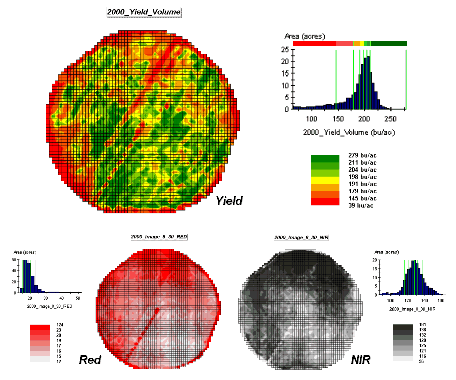
Figure 1.
The corn yield map (top) identifies the pattern to predict; the red and
near-infrared maps (bottom) are used to build the spatial relationship.
While it is difficult for you to assess the subtle relationships between corn yield and the red and near-infrared images, the computer “sees” the relationship quantitatively. Each grid location in the analysis frame has a value for each of the map layers— 3,287 values defining each geo-registered map covering the 189-acre field.
For example, top portion of figure 2 identifies that the example location has a “joint” condition of red equals 14.7 counts and yield equals 218 bu/ac. The red lines in the scatter plot on the right show the precise position of the pair of map values—X= 14.7 and Y= 218. Similarly, the near-infrared and yield values for the same location are shown in the bottom portion of the figure.
In fact the set of “blue dots” in both of the scatter plots represents data pairs for each grid location. The blue lines in the plots represent the prediction equations derived through regression analysis. While the mathematics is a bit complex, the effect is to identify a line that “best fits the data”— just as many data points above as below the line.
In a sense, the line sort of identifies the average yield for each step along the X-axis (red and near-infrared responses respectively). Come to think of it, wouldn’t that make a reasonable guess of the yield for each level of spectral response? That’s how a regression prediction is used… a value for red (or near-infrared) in another field is entered and the equation for the line is used to predict corn yield. Repeat for all of the locations in the field and you have a prediction map of yield from an aerial image… but alas, if it were only that simple and exacting.
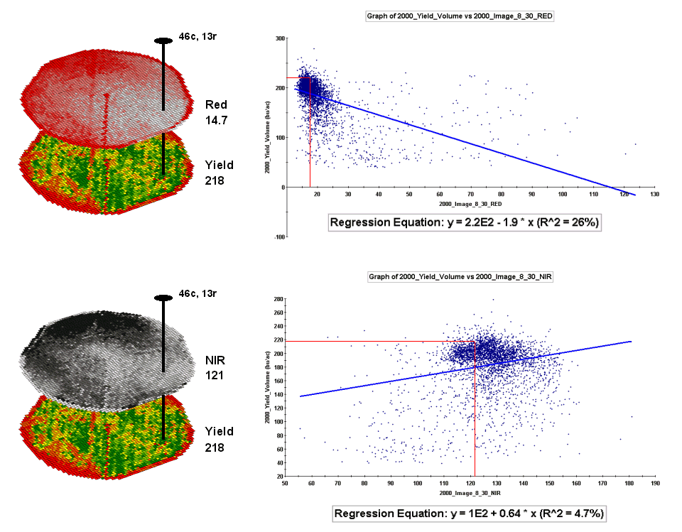
Figure 2.
The joint conditions for the spectral response and corn yield maps are
summarized in the scatter plots shown on the right.
A major problem is that the “r-squared” statistic for both of the prediction equations is fairly small (R^^2= 26% and 4.7% respectively) which suggests that the prediction lines do not fit the data very well. One way to improve the predictive model might be to combine the information in both of the images. The “Normalized Density Vegetation Index (NDVI)” does just that by calculating a new value that indicates plant vigor— NDVI= ((NIR – Red) / (NIR + Red)).
Figure 3 shows the process for calculating NDVI for the sample grid location— ((121-14.7) / (121 + 14.7))= 106.3 / 135.7= .783. The scatter plot on the right shows the yield versus NDVI plot and regression line for all of the field locations. Note that the R^^2 value is a higher at 30% indicating that the combined index is a better predictor of yield.
The bottom portion of the figure evaluates the prediction equation’s performance over the field. The two smaller maps show the actual yield (left) and predicted yield (right). As you would expect the prediction map doesn’t contain the extreme high and low values actually measured.
However the larger map on the right calculates the error of the estimates by simply subtracting the actual measurement from the predicted value at each map location. The error map suggests that overall the yield “guesses” aren’t too bad— average error is a 2.62 bu/ac over guess; 67% of the field is within 20 bu/ac. Also note that most of the over estimating occurs along the edge of the field while most of the under estimating is scattered along curious NE-SW bands.
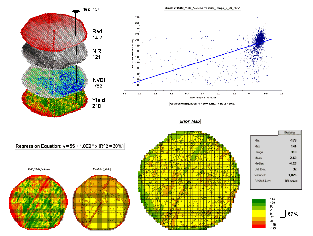
Figure 3. The red and NIR
maps are combined for NDVI value that is a better
predictor of yield.
While evaluating
a prediction equation on the data that generated it isn’t validation, the
procedure provides at least some empirical verification of the technique. It suggests a glimmer of hope that with some
refinement the prediction model might be useful in predicting yield before
harvest. Next month we’ll investigate
some of these refinement techniques and see what information can be gleamed by
analyzing the error surface.
Stratify Maps to Make Better Predictions
(GeoWorld,
February 2002, pg. 20-21)
The previous section described procedures for predictive analysis of mapped data. While the underlying theory, concerns and considerations can easily consume a graduate class for a semester the procedure is quite simple. The grid-based processing preconditions the maps so each location (grid cell) contains the appropriate data. The “shishkebab” of numbers for each location within a stack of maps are analyzed for a prediction equation that summarizes the relationships.
In the example
discussed last month, regression analysis was used to relate a map of NDVI (“normalized density vegetation index” derived from
remote sensing imagery) to a map of corn yield for a farmer’s field. Then the equation was used to derive a map of
predicted yield based on the NDVI values and the
results evaluated for how well the prediction equation performed.
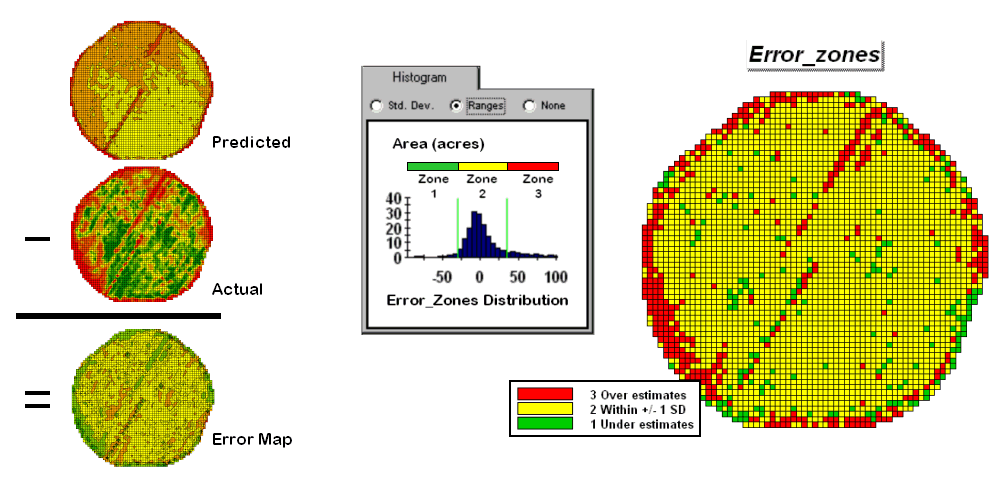
Figure 1. A field can be stratified based on prediction
errors.
The left side of figure 1 shows the evaluation procedure. Subtracting the actual yield values from the predicted ones for each map location derives an Error Map. The previous discussions noted that the yield “guesses” weren’t too bad—average error of 2.62 bu/ac with 67% of the estimates within 20 bu/ac of the actual yield. However, some locations were as far off as 144 bu/ac (over-guess) and –173 bu/ac (under-guess).
One way to improve the predictions is to stratify the data set by breaking it into groups of similar characteristics. The idea is that set of prediction equations tailored to each stratum will result in better predictions than a single equation for an entire area. The technique is commonly used in non-spatial statistics where a data set might be grouped by age, income, and/or education prior to analysis. In spatial statistics additional factors for stratifying, such as neighboring conditions and/or proximity, can be used.
While there are several alternatives for stratifying, subdividing the error map will serve to illustrate the conceptual approach. The histogram in the center of figure 1 shows the distribution of values on the Error Map. The vertical bars identify the breakpoints at plus/minus one standard deviation and divide the map values into three strata—zone 1 of unusually high under-guesses (red), zone 2 of typical error (yellow) and zone 3 of unusually high over-guesses (green). The map on the right of the figure locates the three strata throughout the field.
The rationale behind the stratification is that the whole-field prediction equation works fairly well for zone 2 but not so well for zones 1 and 3. The assumption is that conditions within zone 1 makes the equation under estimate while conditions within zone 3 cause it to over estimate. If the assumption holds one would expect a tailored equation for each zone would be better at predicting than an overall equation. Figure 2 summarizes the results of deriving and applying a set of three prediction equations.
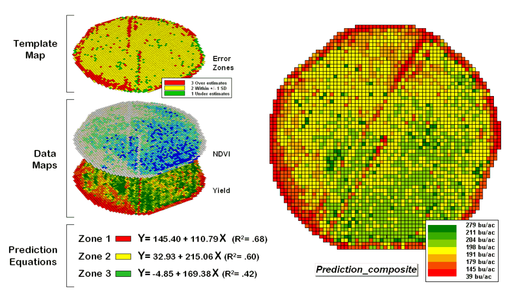
Figure 2. After stratification, prediction equations
can be derived for each element.
The left side of the figure illustrates the procedure. The Error Zones map is used as a template to identify the NDVI and Yield values used to calculate three separate prediction equations. For each map location, the algorithm first checks the value on the Error Zones map then sends the data to the appropriate group for analysis. Once the data has been grouped a regression equation is generated for each zone. The “r-squared” statistic for all three equations (.68, .60, and .42 respectively) suggests that the equations fit the data fairly well and ought to be good predictors. The right side of figure 2 shows the composite prediction map generated by applying the equations to the NDVI data respecting the zones identified on the template map.
The left side of figure 3 provides a visual comparison between the actual yield and predicted maps. The “stratified prediction” shows detailed estimates that more closely align with the actual yield pattern than the “whole-field” derived prediction map. The error map for the stratified prediction shows that eighty percent of the estimates are within +/- 20 bushels per acre. The average error is only 4 bu/ac with maximum under and over-estimates of –81.2 and 113, respectively. All in all, not bad guessing of yield based on a remote sensing shot of the field nearly a month before the field was harvested.
A couple of things should be noted from this example of spatial data mining. First, that there is a myriad of other ways to stratify mapped data—1) Geographic Zones, such as proximity to the field edge; 2) Dependent Map Zones, such as areas of low, medium and high yield; 3) Data Zones, such as areas of similar soil nutrient levels; and 4) Correlated Map Zones, such as micro terrain features identifying small ridges and depressions. The process of identifying useful and consistent stratification schemes is an emerging research frontier in the spatial sciences.
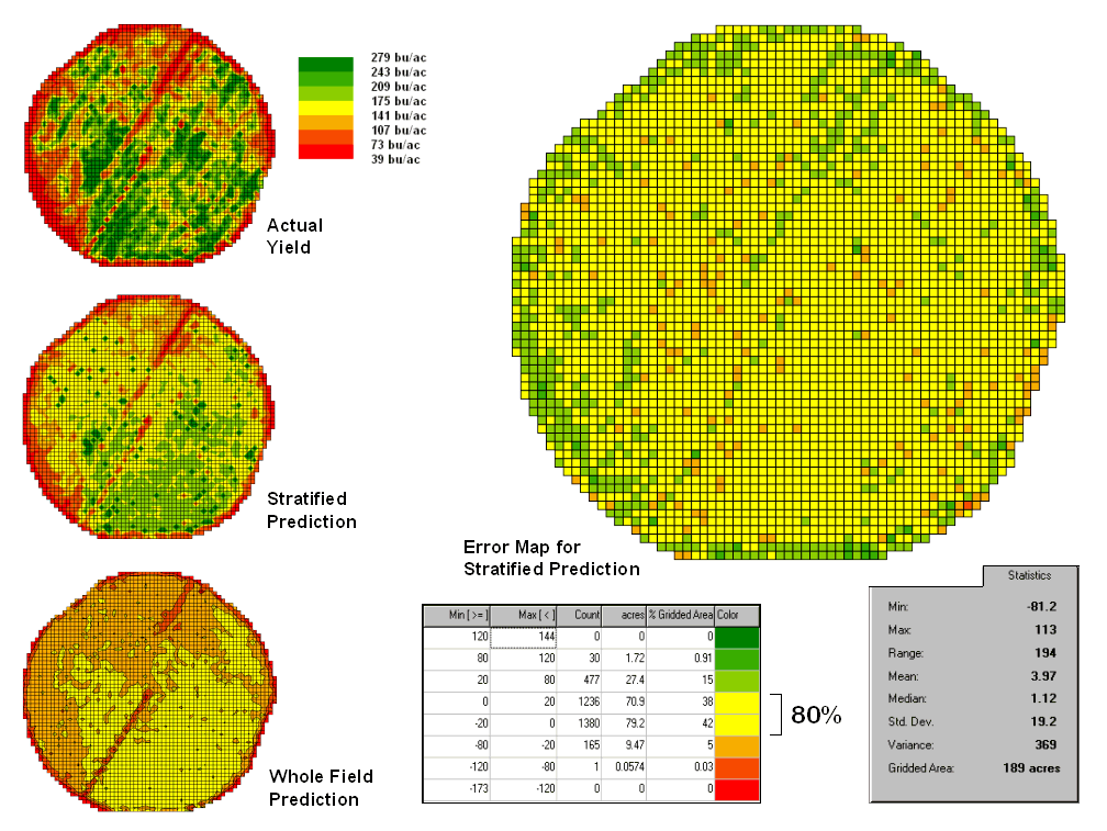
Figure 3. Stratified and whole-field predictions can be
compared using statistical techniques.
Second, the error map is key in evaluating and refining the prediction equations. This point is particularly important if the equations are to be extended in space and time. The technique of using the same data set to develop and evaluate the prediction equations isn’t always adequate. The results need to be tried at other locations and dates to verify performance. While spatial data mining methodology might be at hand, good science is imperative.
Finally, one needs to recognize that spatial data mining is
not restricted to precision agriculture but has potential for analyzing
relationships within almost any set of mapped data. For example, prediction models can be
developed for geo-coded sales from demographic data or timber production
estimates from soil/terrain patterns.
The bottom line is that maps are increasingly seen as organized sets of
data that can be map-ematically analyzed for spatial
relationships… we have only scratched the surface.
_________________