Beyond Mapping III
|
Map
Analysis book with companion CD-ROM for hands-on exercises and further reading |
Beware the
Slippery Surfaces of GIS Modeling
— discusses the
relationships among maps, map surfaces and data distributions
Link Data
and Geographic Distributions — describes
the direct link between numeric and geographic distributions
Normally Things Aren’t Normal — discusses
the appropriateness of using traditional “normal” and percentile statistics
Explore Mapped Data— describes
creation of a Standardized Map Variable surface using Median and
Babies and Bath Water — discusses
the information lost in aggregating field data and assigning typical values to
polygons (desktop mapping)
Explore
Data Space — establishes
the concept of "data space" and how mapped data conforms to this
fundamental view
Identify Data
Patterns — discusses
data clustering and its application in identifying spatial patterns
Note: The processing and figures discussed in this topic were derived using MapCalcTM
software. See www.innovativegis.com to download a
free MapCalc Learner version with tutorial materials for classroom and
self-learning map analysis concepts and procedures.
<Click here> right-click
to download a printer-friendly version of this topic (.pdf).
(Back to the Table of Contents)
______________________________
Beware the Slippery Surfaces of
(GeoWorld, May 1998, pg. 26)
The problem is the traditional paradigm doesn’t fit a lot of reality. Sure the lamppost, roadway and the parking
lot at the mall are physical realities of a map’s set of points, lines and
polygons. Even very real (legally),
though non-physical, property boundaries conceptually align with the
traditional paradigm. But not everything
in space can be so discretely defined, nor is it as easily put in its place.
Obviously meteorological gradients, such as temperature and barometric
pressure, don’t fit the P, L and P mold.
They represent phenomena that are constantly changing in geographical
space, and are inaccurately portrayed as contour lines, regardless how
precisely the lines are drawn. By its
very nature, a continuous spatial variable is corrupted by artificially
imposing abrupt transitions. The contour
line is simply a mechanism to visually portray a 2-dimensional rendering of a
3-dimensional gradient. It certainly
isn’t a basic map feature, nor should it be a data structure for storage of
spatially complex phenomena.
Full-featured
While a contour map of elevation lets your eye assess slope (closeness of
lines) and aspect (downhill direction), it leaves the computer without a clue,
as all it can see is a pile of numbers (digital data), not an organized set of
lines (analog image).
Figure 1 links different views of surface data.
Keep in mind, that the computer doesn’t “see” any of them; they’re for
human viewing enjoyment. The traditional
2-D map view chooses a map value,
then identifies all of the locations (mathematically implied) having that
value. That begs the traditional
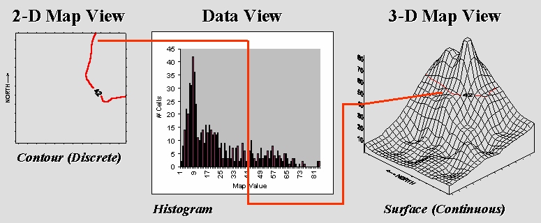
Figure 1. A
histogram (numerical distribution) is linked to a map surface (geographic
distribution) by a common axsis of map values.
However, it’s the discrete nature of a contour map and the irregular
features spawned that restrict its ability to effectively represent continuous
phenomena. The data view uses a histogram to characterize a continuum of map values
in “numeric” space. It summarizes the
number of times a given value occurs in a data set (relative frequency).
The 3-D
map view forms a continuous surface by introducing a regular grid over
an area. The X and Y axes position the
grid cells in geographic space, while the Z axis reports the numeric value at
that location. Note that the data and
surface views share a common axis—map value.
It serves as the link between the two perspectives. For example, the data view shows number of
occurrences for the value 42 and the relative numerical frequency considering
the occurrences for all other values.
Similarly, the surface view identifies all of the locations having a
value of 42 and the relative geographic positioning considering the occurrences
for all other values.
The concept of an “aggregation interval” is shared as well. In constructing a histogram, a constant data
step is used. In the example, a data
interval of 1.0 unit was used, and all fractional values were rounded, then
“placed” in the appropriate “bin.” In an
analogous fashion, the aggregation interval for constructing a surface uses a
constant geographic step, as well as a constant data step. In the example, an interval of 1.0 hectare
was used to establish the constant partitioning in geographic space. In either case, the smaller the aggregation
interval the better the representation.
Both perspectives
characterize data dispersal. The numeric
distribution of data (a histogram’s shape of ups/downs) forms the
cornerstone of traditional statistics and determines appropriate data analysis
procedures. In a similar fashion, a map
surface establishes the geographic distribution of data (a
surface’s shape of hills/valleys) and is the cornerstone of spatial
statistics. The assumptions, linkages,
similarities and differences between these two perspectives of data
distribution are the focus of the next few columns… we’ll dust off the old stat
book together.
Link Data and Geographic
Distributions
(GeoWorld, June 1998, pg. 28-30)
Some of the previous Beyond Mapping articles might have found you
reaching for your old Stat 101 textbook.
Actually, the concepts used in mapped data analysis are quite
simple—it’s the intimidating terminology and “picky, picky” theory that are
hard. The most basic concept involves a number
line that is like a ruler with tic-marks for numbers from small to
large. However, the units aren’t always
inches, but data units like number of animals or dollars of sales. If you placed a dot for each data measurement
(see top of figure 1), there would be a minimum value on the left (#animals
= 0) extending to a maximum value on the right.
The rest of the points would fall on top of each other throughout the
data range.
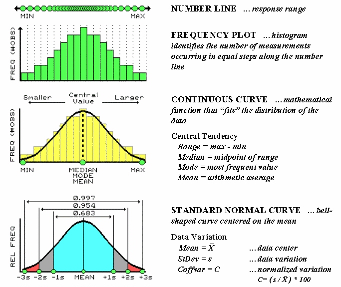
Figure 1. The distribution of measurements in “data
space” is described by its histogram and summarized by descriptive statistics.
To visualize these data, we can look at the number line from the side
and note where the measurements tend to pile up. If the number line is divided into equally
spaced “shoots” (like in pinball machine) the measurements will pile up to form
a histogram
plot of the data’s distribution.
Now you can easily see that most of the measurements fell about
midrange.
In statistics, several terms are used to describe this plot and its “central
tendency.” The median identifies the
“midway” value with half of the distribution below it and half above it, while
the mode
identifies the most frequently occurring value in the data set. The mean, or average, is a bit trickier as it requires calculation. The total of all the measurements is
calculated and then divided by the number of measurements in the data set.
Although the arithmetic is easy (for a tireless computer), its
implications are theoretically deep. When you calculate the mean and its
standard deviation you’re actually imposing the “standard normal curve”
assumption onto the histogram. The
bell-shaped curve is symmetrical with the mean at its center. For the “normally distributed” data shown in
the figure, the fit is perfect with exactly half of the data on either side. Also note that the mean, mode and median
occur at the same value for this idealized distribution of data.
Now let’s turn our attention to the tough stuff—characterizing the data
variation about the mean. When
considering variation one must confront the concept of a standard deviation (StDev). The standard
deviation describes the dispersion, or spread, of the data around the
mean. It’s a consistent measure of the
variation, as one standard deviation on either side of the mean “captures”
slightly more than two-thirds of the data (.683 of the total area under the
curve to be exact). Approximately 95% of
all the measurements are included within two standard deviations, and more than
99% are covered by three.
The larger the standard deviation, the more variable is the data, indicating
that the mean isn’t very typical. In
So what determines whether a standard deviation is large or small? That’s the role of the coefficient of variation
(Coffvar).
This semantically-challenging mouthful simply “normalizes” the variation
in the data by expressing the standard deviation as a percent of the mean—if
it’s large, say over 50%, then there is a lot of variation and the mean is a
poor estimator of what’s happening in a mapped area. Keep this in mind the next time you assign an
average value to map features, such as the average tree diameter for each
forest parcel, or the average home value for each county.
A large portion of the variation
can be “explained” through its spatial distribution. Figure 2 shows a technique that brings statistics
down to earth by mapping the standard normal curve in geographic space. The procedure first calculates the mean and
standard deviation for the typical response in a data set. The data is then spatially interpolated into
a continuous geographic distribution. A standard
normal variable surface is derived by subtracting the mean from the map
value at each location (deviation from the typical), then dividing by the
standard deviation (normalizing to the typical variation) and multiplying by a
hundred to form a percent. The result is
that every map location gets a number indicating exactly how “typical” it is.
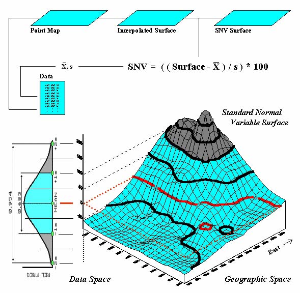
Figure 2. A
“standard normal surface” identifies how typical every location is for an area
of interest.
The contour lines draped on the
Normally Things Aren’t
(GeoWorld, September 2007, pg. 18)
No matter how hard
you have tried to avoid the quantitative “dark” side of GIS, you likely have
assigned the average (Mean) to a set of data
while merrily mapping it. It might have
been the average account value for a sales territory, or the average visitor
days for a park area, or the average parts per million of phosphorous in a
farmer’s field. You might have even
calculated the Standard Deviation to
get an idea of how typical the average truly was.
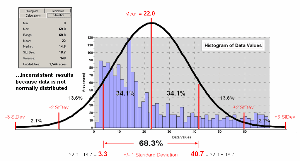
Figure 1. Characterizing data distribution as +/- 1 Standard
Deviation from the Mean.
But there is a major
assumption every time you map the average—that the data is Normally Distributed. That
means its histogram approximates the bell curve shape you dreaded during
grading of your high school assignments.
Figure 1 depicts a standard normal curve applied to a set of spatially
interpolated animal activity data.
Notice that the fit is not too good as the data distribution is
asymmetrical—a skewed condition typical of most data that I have encountered in
over 30 years of playing with maps as numbers.
Rarely are mapped data normally distributed, yet most map analysis
simply sallies forth assuming that it is.
A key point is that the vertical axis of the histogram for spatial data indicates geographic area covered by each increasing response step along the horizontal axis. If you sum all of the piecemeal slices of the data it will equal the total area contained in the geographic extent of a project area. The assumption that the areal extent is symmetrically distributed in a declining fashion around the midpoint of the data range hardly ever occurs. The norm is ill-fitting curves with infeasible “tails” hanging outside the data range like the baggy pants of the teenagers at the mall.
As “normal” statistical analysis is applied to multiple skewed data sets (the spatial data norm) comparative consistency is lost. While the area under the standard normal curve conforms to statistical theory, the corresponding geographic area varies widely from one map to another.
Figure 2 depicts an alternative technique involving percentiles. The data is rank-ordered (either ascending or descending) and then divided into Quartiles with each step containing 25% of the data. The Median identifies the breakpoint with half of the data below and half above. Statistical theory suggests that the mean and median align for the ideal normal distribution. In this case, the large disparity (22.0 versus 14.6) confirms that the data is far from normally distributed and skewed toward lower values since the median is less than the mean. The bottom line is that the mean is over-estimating the true typical value in the data (central tendency).
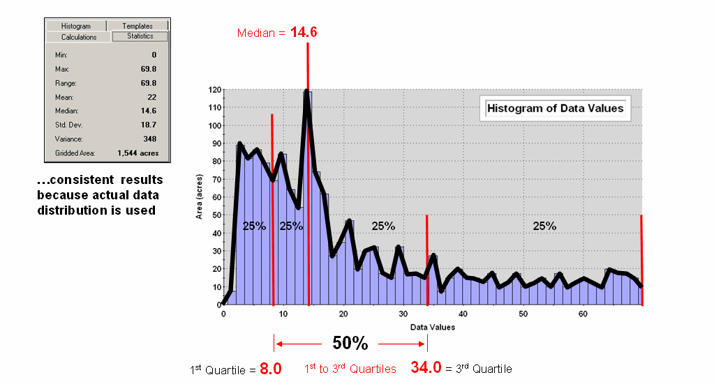
Figure 2. Characterizing data distribution as +/- 1 Quartile
from the Median.
Notice that the quartile breakpoints vary in width responding to the actual distribution of the data. The interpretation of the median is similar to that of the mean in that it represents the central tendency of the data. In an analogous manner, the 1st to 3rd quartile range is analogous to +/- 1 standard deviation in that it represents the typical data dispersion about the typical value.
What is different is that the actual data distribution is respected and the results always fit the data like a glove. Figure 3 maps the unusually low (blue) and high (red) tails for both approaches—traditional statistics (a) and percentile statistics (b). Notice in inset a) that the low tail is truncated as the fitted normal curve assumes that the data can go negative, which is an infeasible condition for most mapped data. In fact most of the low tail is lost to the infeasible condition, effectively misrepresenting the spatial pattern of the unusually low areas. The 2D discrete maps show the large discrepancy in the geographic patterns.

Figure 3. Geographic patterns resulting from the two thematic
mapping techniques.
The astute reader will recognize that the percentile statistical approach is the same as the “Equal Counts” display technique used in thematic mapping. The percentile steps could even be adjusted to match the + /- 34.1, 13.6 and 2.1% groupings used in normal statistics. Discussion in the next section builds on this idea to generate a standard variable map surface that identifies just how typical each map location is—based on the actual data distribution, not an ill-fitted standard normal curve …pure heresy.
(GeoWorld, October, 2007)
The discussion
suggested an alternative statistic, the Median,
as a much more stable central tendency measure.
It is identifies the break point where half of the data is below and
half is above ...analogous to the Average.
A measure of data variation is formed by identifying the Quartile Range from the lowest 25% of
the data (1st quartile) and the uppermost 25% (4th
quartile) …analogous to the Standard Deviation.
The approach consistently recognizes the actual balance point for mapped
data and never force-fits a solution outside of the actual data range.
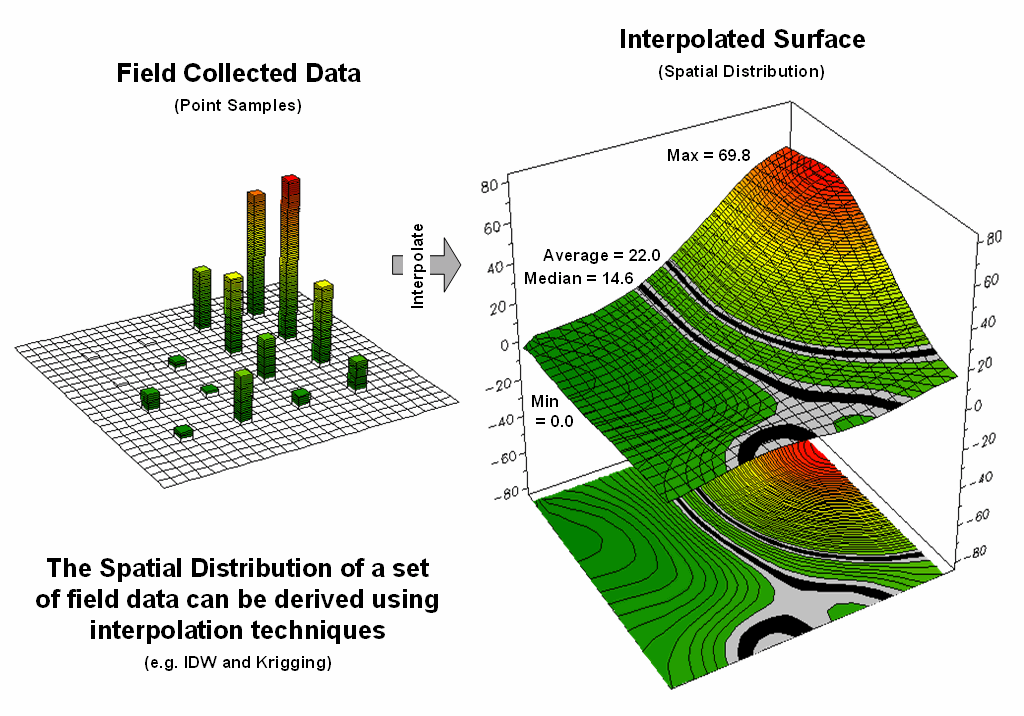
Figure
1.
Spatial Interpolation is used to generate the spatial distribution
(continuous surface) inherent in a set of field data (discrete points).
This section takes
the discussion a bit further by generating a Standardized Map Variable surface that identifies just how typical
each map location is based on the actual data distribution, not an ill-fitted
standard normal curve. Figure 1 depicts the first step of the
process involving the conversion of the discrete point data into its implied
spatial distribution. Notice that the
relatively high sample values in the NE form a peak in the surface, while the
low values form a valley in the NW.
Both the Average and
Median are shown in the surface plot on the right side of the figure. As discussed in the last section, the Average
tends to over-estimate the typical value (central tendency) because the
symmetric assumption of the standard normal curve “slops” over into infeasible
negative values. This condition is graphically
reinforced in the figure by noting the lack of spatial balance between the area
above and below the Average. The Median,
on the other hand, balances just as much of the project area above the Median
as below.
Figure 2 extends
this relationship by generating a Standardized
Map Variable surface. The
calculation normalizes the difference between the interpolated value at each
location and the Median using the equation shown in the figure (where Q_Range is the
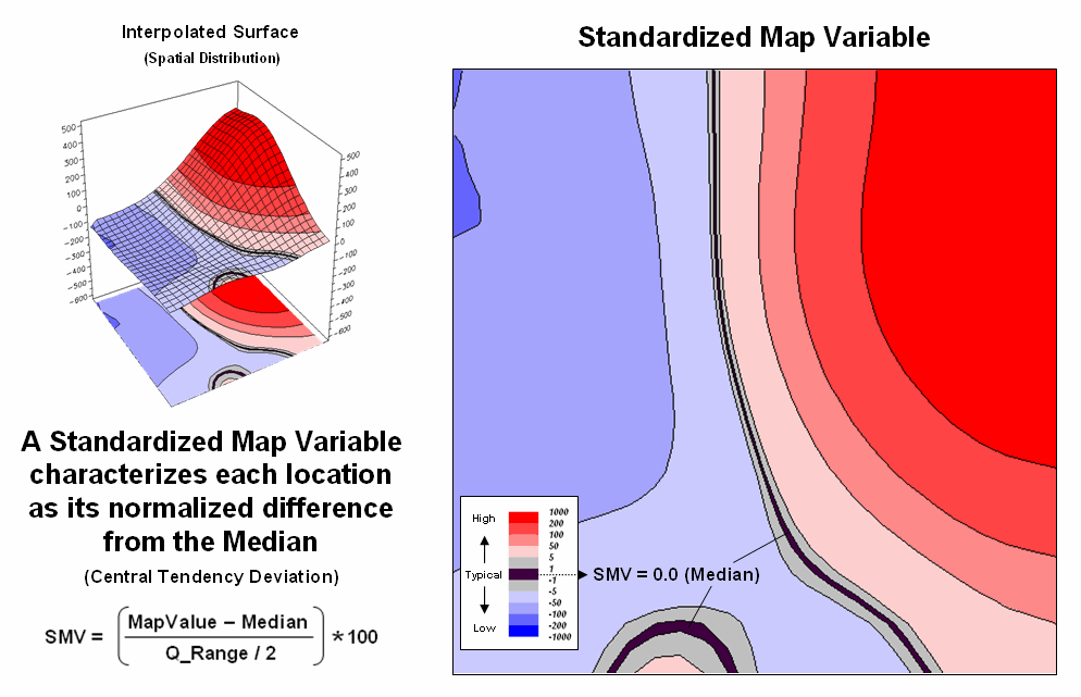
Figure
2. A
Standardized Map Variable (SMV) uses the Median and
The real value of
viewing your field collected data as a Standardized Map Variable (SMV) is that
is consistent for all data. You have
probably heard that you can’t compare “apples and oranges” but with a SMV
surface you can. Figure 3 shows the
results for two different variables for the same project area.
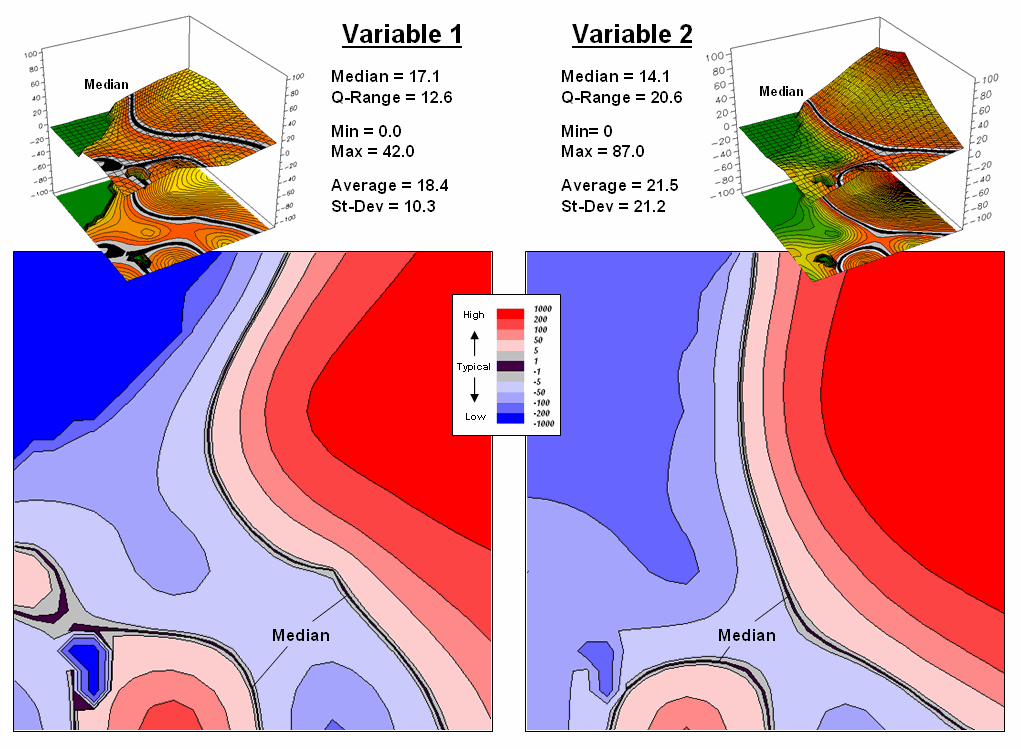
Figure
3.
Mapping the spatial distribution of field data enables discovery of
important geographic patterns that are lost when the average is assigned to
entire spatial objects.
SMV normalization
enables direct comparison as percentages of the typical data dispersion within
data sets and without cartographic confusion and inconsistency. A dark red area is just as unusually high in
variable 1 as it is in variable 2, regardless of their respective measurement
units, numerical distribution or spatial distribution.
That means you can
get a consistent “statistical picture” of the relative spatial distributions (where
the low, typical and high values occur) among any mapped data sets you might
want explore. How the blue and red color
gradients align (or don’t align) provides considerable insight into common
spatial relationships and patterns of mapped data.
(GeoWorld, November, 2007)
This section takes
the discussion to new heights (or is it lows?) by challenging the use of any
scalar central tendency statistic to represent mapped data. Whether the average or the median is used, a
robust set of field data is reduced to a single value assumed to be same
everywhere throughout a parcel. This
supposition is the basis for most desktop mapping applications that takes a set
of spatially collected data (parts per million, number of purchases, disease
occurrences, crime incidence, etc.), reduces all of the data to a single value
(total, average, median, etc.) and then “paints” a fixed set of polygons with
vibrant colors reflecting the scalar statistic of the field data falling within
each polygon.
For example, the
left side of figure 1 depicts the position and relative values of some field
collected data; the right side shows the derived spatial distribution of the
data for an individual reporting parcel.
The average of the mapped data is shown as a superimposed plane
“floating at average height of 22.0” and assumed the same everywhere within the
polygon. But the data values themselves,
as well as the derived spatial distribution, suggest that higher values occur
in the northeast and lower values in the western portion.
Figure
1. The
average of a set of interpolated mapped data forms a uniform spatial
distribution (horizontal plane) in continuous 3D geographic space.
The first thing to notice
in figure 1 is that the average is hardly anywhere, forming just a thin band
cutting across the parcel. Most of the
mapped data is well above or below the average.
That’s what the standard deviation attempts to tell you—just how typical
the computed typical value really is. If
the dispersion statistic is relatively large, then the computed typical isn’t
typical at all. However, most desktop
mapping applications ignore data dispersion and simply “paint” a color
corresponding to the average regardless of numerical or spatial data patterns
within a parcel.
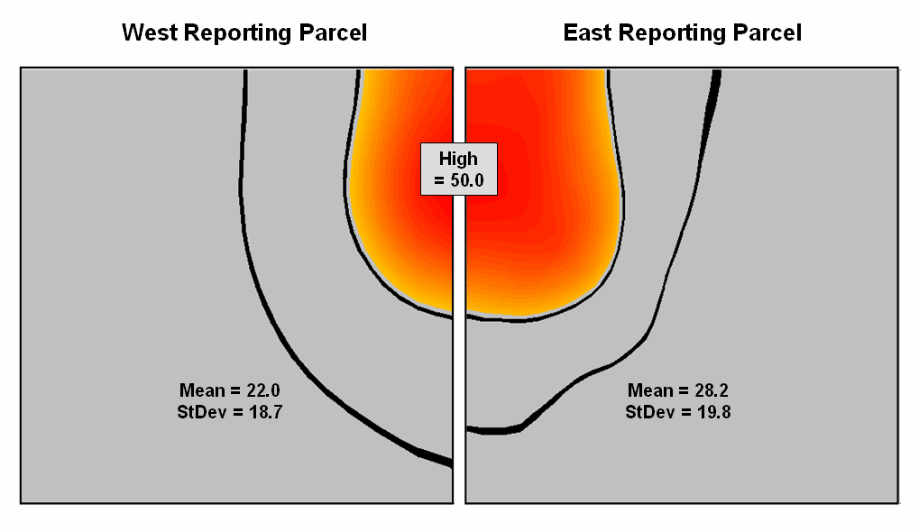
Figure 2 shows how
this can get you into a lot of trouble.
Assume the data is mapping an extremely toxic chemical in the soil that,
at high levels, poses a serious health risk for children. The mean values for both the West (22.0) and
the East (28.2) reporting parcels are well under the “critical limit” of
50.0. Desktop mapping would paint both
parcels a comfortable green tone, as their typical values are well below
concern. Even if anyone checked, the
upper-tails of the standard deviations don’t exceed the limit (22.0 + 18.7=
40.7 and 28.2 + 19.8= 48.0). So from a
non-spatial perspective, everything seems just fine and the children aren’t in
peril.
Figure
2. Spatial distributions and superimposed average planes for two
adjacent parcels.
Figure 3, however,
portrays a radically different story. The
West and East map surfaces are sliced at the critical limit to identify areas
that are above the critical limit (red tones).
The high regions, when combined, represent nearly 15% of the project
area and likely extend into other adjacent parcels. The aggregated, non-spatial treatment of the
spatial data fails to uncover the pattern by assuming the average value was the
same everywhere within a parcel.
Figure
3.
Mapping the spatial distribution of field data enables discovery of
important geographic patterns that are lost when the average is assigned to
entire spatial objects.
Our paper mapping
legacy leads us to believe that the world is composed of a finite set of
discrete spatial objects—county boundaries, administrative districts, sales
territories, vegetation parcels, ownership plots and the like. All we have to do is color them with data
summaries. Yet in reality, few of these
groupings provide parceling that reflects inviolate spatial patterns that are
consistent over space and time with every map variable. In a sense, a large number of GIS
applications “throw the baby (spatial distribution) out with the bath water
(data)” by reducing detailed and expensive field data to a single, maybe or
maybe not, typical value.
(GeoWorld, July 1998, pg. 28)
Following my usual recipe for journalistic suicide let’s consider the
fundamental concepts of the dismal discipline of spatial statistics within the
context of production agriculture. For
example, a map of phosphorous in the top layer of soil (0-5cm) in a farmer’s
field contains values ranging from 22 to 140 parts per million. The spatial pattern of these data is
characterized by the relative positioning of the data values within a reference
grid of cell locations. The set of cells
forming the analysis grid identifies the spatial domain (geographic space), while
the map values identifies the data domain (data space).
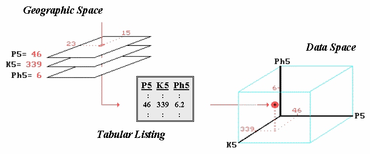
Figure 1. The
map values for a series of maps can be simultaneously plotted in data space.
A dull and tedious tabular listing, as shown in the
center of Figure 1, is the traditional human perspective of such data. We can’t consume a long list of numbers, so
we immediately turn the entire column of data into a single “typical” value
(average) and use it to make a decision.
For the soil phosphorous data set, the average is 48. A location in the center of the field (column
15, row 23 of the analysis grid) has a phosphorous level of 46 that is close to
the average value (in a data sense, not a geographic sense). But recall that the data range tells us that
somewhere in the field there is at least one location that is less than half
(22) and another that is nearly three times the average (140), so the average
value doesn’t tell it all.
Now consider additional map surfaces of potassium levels (K5) and soil acidity
(Ph5), as well as phosphorous (P5), for the field. As humans we could “see” the coincidence of
these data sets by aligning their long columns of numbers in a spreadsheet or
database. Specific levels for all three
of the soil measurements at any location in the field are identified as rows in
the table. However, the combined set of
data is even more indigestible, with the only “humane” view of map coincidence
being the assumption that the averages are everywhere— 48, 419, 6.2 in this
example. The center location’s data
pattern of 46, 339, and 6.0 is fairly similar to the pattern of the
field averages, but exactly how similar?
Which map locations in the field are radically different?
Before we can answer these questions, we need to understand how the computer
“sees” similarities and differences in multiple sets of data. It begins with a three-dimensional plot in
data space as shown on the right side of figure 1. The data values along a row of the tabular
listing are plotted resulting in each map location being positioned in the
imaginary box based on its data pattern.
Similarity among the field’s soil response patterns are determined by
their relative positioning in the box— locations that plot to the same position
in the data space box are identical; those that plot farther away from one
another are less similar.
How the computer “measures” the relative distance becomes the secret ingredient
in assessing data similarity. Actually
it’s quite simple if you revisit a bit of high school geometry, but I bet you
thought you had escaped all that awful academic fluff when you entered the
colorful, fine arts world of computer mapping and geo-query.
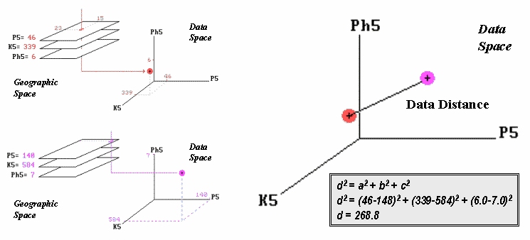
Figure 2.
Similarity is determined by the data distance between two locations and
is calculated by expanding the Pythagorean Theorem.
The left side of figure 2 shows the
data space plots for soil conditions at two locations in the farmer’s
field. The right side of the figure
shows a straight line connecting the data points whose length identifies the
data distance between the points. Now
for the secret— it’s the old Pythagorean theorem of c2 = a2
+ b2 (I bet you remember it).
However, in this case it looks like d2 = a2 + b2
+ c2 as it has to be expanded to three dimensions to accommodate the
three maps of phosphorous, potassium and acidity (P5, K5 and Ph5 axes in the
figure). All that the Wizard of Oz
(a.k.a., computer programmer) has to do is subtract the values for each
condition between two locations and plug them into the equation. If there are more than three maps, the
equation simply keeps expanding into hyper-data
space which as humans we can no longer plot or easily conceptualize.
(GeoWorld, August 1998, pg. 26-27)
The previous section introduced the concept of data distance. While most of us are comfortable with the
concept of distance in geographic space, things get a bit abstract when we move
from feet and meters in the real world to data units in data space.
Recall that data space is formed by the intersection of two or more axes in a
typical graph. If you measured the
weight and height of several students in your old geometry class, each of the
paired measurements for a person would plot as a dot in XY data space locating
their particular weight (X axis) and height (Y axis) combination. A plot of all the data looks like a shotgun
blast and is termed a scatter plot.
The scatter plots for a lot of data sets form clusters of similar
measurements. For example, two distinct
groups might be detected in the geometry class’s data—the demure cheerleaders
(low weight and height) and the football studs (high weight and height). Traditional (non-spatial) data analysis stops
at identifying the groupings. Spatial
statistics, however, extends the analysis to geographic contexts.
If seating “coordinates” accompanied the classroom data you might detect that
most of the cheerleaders were located in one part of the room, while the studs
were predominantly in another. Further
analysis might show a spatial relation between the positioning of the groups
and proximity of the teacher—cheerleaders in front and studs in back.
The linking of traditional statistics with spatial analysis capabilities (such
as proximity measurement) provides insight into the spatial context and
relationships inherent in the data. The
only prerequisite is “tagging” geographic coordinates to the measurements. Until recently, this requirement presented
quite a challenge and spatial coordinates were rarely included in most data
sets. With the advent of
The new hurdle, however, isn’t so much technical as it is social. Most data analysis types aren’t familiar with
spatial concepts, while most
The scatter plot in inset (a) of figure 1 shows weight/height
data that might have been collected in your old geometry class. Note that all of the students do not have the
same weight/height measurements and that many vary widely from the class average. Your eye easily detects two groups (low/low
and high/high) in the plot but the computer just sees a bunch of numbers. So how does it identify the groups without
seeing the scatter plot?
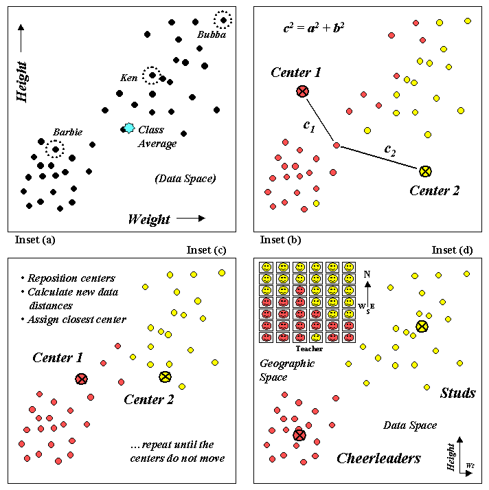
Figure 1.
Clustering uses repeated data distance calculations to identify
numerical patterns in a data set.
One approach (termed k-means
clustering) arbitrarily establishes two cluster centers in the data space
(inset (b)). The data distance to each
weight/height measurement pair is calculated and the point is assigned to the
closest cluster center. Recall from last
month’s article that the Pythagorean theorem of c2
= a2 + b2 is used to calculate the data distance and can be
extended to more than just two variables (hyper-data space). It should be at least some comfort to note
that the geometry you learned in high school holds for the surreal world of
data space, as well as the one you walk on.
In the example, c1
is smaller than c2
therefore that student’s measurement pair is assigned to cluster center 1. The remaining student assignments are
identified in the scatter plot by their color codes.
The next step calculates the average weigh/height of the assigned
students and uses these coordinates to reposition the cluster centers (inset
(c)). Other rounds of data distances,
cluster assignments and repositioning are made until the cluster membership
does not change (i.e., the centers do not move).
Inset (d) shows the final groupings with the big folks (high/high)
differentiated from the smaller folks (low/low). By passing these results to a
The positioning of these data in the real world classroom (upper left portion
of inset (d)) shows a distinct spatial pattern between the two
groups—smaller folks in front and bigger folks in the rear. Like before, you simply see these things but
the computer has to derive the relationships (distance to similar neighbor)
from a pile of numbers.
What is important to note is that analysis in data space and geographic space
has a lot in common. In the example,
both “spaces” are represented as XY coordinates—weight/height measurements in
data space (characteristics) and longitude/latitude in geographic space
(positioning). Data distance is used to
partition the measurements into separate groups (data pattern). Geographic distance is used to partition the
locations into separate groups (spatial pattern). In both instances the old Pythagorean Theorem
served as the procedure for measuring distance.
So who cares? We have gotten
along for years with data analysts and mapmakers doing their own thing. Maps are maps and data are data, right? Not exactly, at least not any more… with the
advent of the digital map, maps are data (not pictures). Information on the relative positioning and
coincidence among mapped variables extend traditional data analysis. Likewise, the digital nature of maps provides
data analysis tools that enable us to “see” geographic space in abstract terms
(decision-making) beyond traditional descriptions of precise placement of
physical features (inventory).