|
Topic 8 – The Anatomy of
a GIS Model |
Spatial Reasoning
book |
From
Recipes to Models — describes basic Binary and Rating model
expressions using a simple Landslide Susceptible model
Extending
Basic Models through Logic Modifications — describes logic extensions to
a simple Landslide Susceptible model by adding additional criteria that changes
a model’s structure
Evaluating Map-ematical Relationships — discussed
the differences and similarities between the two basic types of GIS models
(Cartographic and Spatial) using the Universal Soil Loss Equation as an example
<Click here> for a printer-friendly version of this topic
(.pdf).
(Back to the Table of Contents)
______________________________
From Recipes
to Models
(GeoWorld, December 1995)
So
what's the difference between a recipe and a model? Both seem to mix a bunch of things together
to create something else. Both result in
a synergistic amalgamation that's more than the sum of the parts. Both start with basic ingredients and
describe the processing steps required to produce the desired result-be it a
chocolate cake or a landslide susceptibility map.
In a
GIS, the ingredients are base maps and the processing steps are spatial
handling operations. For example, a simple
recipe for locating landslide susceptibility involves ingredients such as
terrain steepness, soil type, and vegetation cover; areas that are steep,
unstable, and bare are the most susceptible.
Before
computers, identifying areas of high susceptibility required tedious manual map
analysis procedures. A transparency was
taped over a contour map of elevation, and areas where contour lines were
spaced closely (steep) were outlined and filled with a dark color. Similar transparent overlays were interpreted
for areas of unstable soils and sparse vegetation from soil and vegetation base
maps. When the three transparencies were
overlaid on a strong light source, the combination was deciphered easily— clear
= not susceptible, and dark = susceptible.
That basic recipe has been with us for a long time. Of course, the methods changed as modern
drafting aids replaced the thin parchment, quill pens, and stained glass
windows of the 1800s, but the conceptual approach remains the same.
In a
typical vector GIS, a logical combination is achieved by first generating a
topological overlay of the three maps (SLOPE, SOILS, COVERTYPE), then querying
the resultant table (Tsv_olv) for susceptible
areas. The Structured Query Language
(SQL) query might look like the following:
Select columns: %slope, Soil_stability,
Covertype
from tables:
TSV_OVL
where condition:
%slope > 13 AND Soil_stability =
"Unstable" AND Covertype = "Bare"
into table named:
L_HAZARD
The flowchart
in figure 1 depicts an alternative raster-based binary model (only two states
of either Yes or No), which mimics the manual map analysis process and achieves
the same result as the overlay/SQL query.
A slope map is created by calculating the change in elevation throughout
the project area (first derivative of the elevation surface).
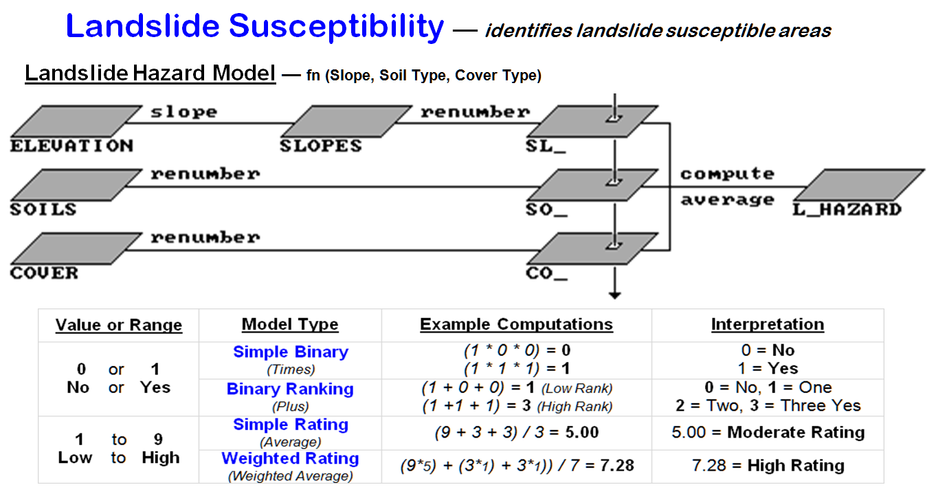
Figure
1. Binary, ranking and rating models of landslide susceptibility. The location indicated by the piercing arrow contains
34 percent slope, a fairly stable soil and sparse forest cover.
A Simple Binary model solution codes as
“1” all of the susceptible areas on each of the factor maps (>30 percent
slope, unstable soils, bare vegetative cover), whereas the non-susceptible
areas are coded as “0.” The product of the three binary maps (SL_HAZARD (binary), SO_ HAZARD (binary), CO_ HAZARD (binary)) creates a final map of
landslide potential— l = susceptible, and 0 = not susceptible. Only locations susceptible on all three maps
retain the "susceptible" classification (1*1*1= l). In the other instances, multiplying 0 times
any number forces the product to 0 (not susceptible). The map-ematical
model corresponding to the flowchart (Simple
Binary model) in figure 1 might be expressed (in TMAP modeling language)
as:
|
SLOPE
ELEVATION FOR SLOPES |
…creates a Slope map, 1- susceptible |
|
RENUMBER SLOPES FoR sl_BINARY ASSIGNING 0 To 1 THRu
12 ASSIGNING
1 TO 13 THRU 1000 |
...identifies >13% as steep, 1= susceptible |
|
RENUMBER SOILS FOR SO__BINARY ASSIGNING 0 TO 0 THRU
2 ASSIGNING I
TO 3 THRU 4 |
…identifies soils 3&4 as unstable, 1=
susceptible |
|
RENUMBER covERTypE FOR co_BINARY ASSIGNING 0 To 1 ASSIGNING 0 To 3 ASSIGNING 1 To 2 |
…identifies cover type 2 as bare= 1 susceptible |
|
coMpuTE
sl__HAZARD TIMES so__HAZARD TIMES co__HAZARD
FoR L_HAZARD |
…computes 1 * 1 * 1 = 1 to identify hazardous
areas |
In the
multiplicative case, the arithmetic combination of the maps yields the original
two states-dark or 1 = susceptible, and clear or 0 = not susceptible (at least
one data layer not susceptible). It's
analogous to the "AND" condition of the logical combination in the
SQL query. However, other combinations
can be derived. For example, the visual
analysis could be extended by interpreting the various shades of gray on the
stack of transparent overlays: clear = not susceptible, light gray = low
susceptibility, medium gray = moderate susceptibility and dark gray = high
susceptibility.
In an
analogous map-ematical approach, the computed sum of
the three binary maps yields a similar ranking: 0 = not susceptible, 1 = low
susceptibility, 2 = moderate susceptibility and 3 = high susceptibility (l + l+
l = 3). That approach is called a Binary Ranking model, because it
develops an ordinal scale of increasing landslide potential— a value of two is
more susceptible than a value of 1, but not necessarily twice as
susceptible.
A
rating model is different, because it uses a consistent scale with more than
two states to characterize the relative landslide potential for various
conditions on each factor map. For
example, a value of 1 is assigned to the least susceptible steepness condition
(e.g., from 0 percent to 5 percent slope), while a value of 9 is assigned to
the most susceptible condition (e.g., >30 percent slope). The intermediate conditions are assigned
appropriate values between the landslide susceptibility extremes of 1 and
9. That calibration results in three
maps with relative susceptibility ratings (SL_HAZARD (rate), SO_HAZARD (rate),
CO_HAZARD (rate)) based on the 1-9
scale of relative landslide susceptibility.
Computing
the simple average (Simple Rating
model) of the three rate maps determines an overall landslide potential based
on the relative ratings for each factor at each map location. For example, a particular grid cell might be
rated 9, because it's steep, 3 because its soil is fairly stable, and I because
it's forested. The average landslide
susceptibility rating under these conditions is [(9+3+3)/3] = 5, indicating a
moderate landslide potential.
A
weighted average of the three maps (Weighted
Rating model) expresses the relative importance of each factor to determine
overall susceptibility. For example,
steepness might be identified as five times more important than either soils or
vegetative cover in estimating landslide potential. For the example grid cell described
previously, the weighted average computes to [([9*5]+3+3)
l7) = 7.28, which is closer to a high overall rating. The weighted average is influenced
preferentially by the SL-rate map's high rating, yielding a much higher overall
rating than the simple average.
All
that may be a bit confusing. The four
different "recipes" for landslide potential produced strikingly different
results for the example grid cell in figure 1— from not susceptible to high
susceptibility. It's like baking banana
bread. Some folks follow the traditional
recipe; some add chopped walnuts or a few cranberries. By the time diced dates and candied cherries
are tossed in, you can't tell the difference between your banana bread and last
years' fruitcake.
So back
to the main point-what's the difference between a recipe and a model? Merely semantics? Simply marketing jargon? The real difference between a recipe and a
model isn't in the ingredients, or the processing steps themselves. It's in the conceptual fabric of the process
…but more on that later.
Extending Basic Models through Logic Modifications
(GeoWorld, January 1996)
The
previous section described various renderings of a landslide susceptibility
model. It related the results obtained
for an example location using manual, logical combination, binary, ranking, and
rating models. The results ranged from
not susceptible to high susceptibility.
Two factors in model expression were at play: the type of model and its
calibration.
However,
the model structure, which identified the factors considered and how they
interact, remained constant. In the
example, the logic was constrained to jointly considering terrain steepness,
soil type, and vegetation cover. One
could argue other factors might contribute to landslide potential. What about depth to bedrock? Or previous surface
disturbance? Or slope length? Or precipitation frequency and intensity? Or gopher population
density? Or about anything else
you might dream up?
That's
it. You've got the secret to
seat-of-the-pants GISing. First you address the critical factors, and
then extend your attention to other contributing factors. In the abstract it means adding boxes and
arrows to the flowchart to reflect the added logic. In practice it means expanding the GIS macro
code, and most importantly wrestling with the model's calibration.
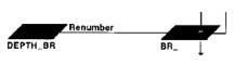
For
example, it's easy to add a fourth row to the landslide flowchart, identifying
the additional criterion of depth to bed rock, and tie it to the other three
factors. It's even fairly easy to add
the new lines of code to the GIS macro (Binary
Ranking model):
|
|
RENUMBER DEPTH_BR assigning 0 to 0 thru 4 assigning 1 to 5 thru 15 For BR_binary |
…identifies depth to bedrock > 4m as minimal
susceptibility = 1 |
|
coMpuTE sl_binary PLUS so_binary PLUS co_binary PLUS br_BINARY FoR L_HAZARD |
…for example: compute 1 + 1 + 1+ 1 = 4 to identify extremely hazardous
areas |
Things
get a lot tougher when you have to split hairs about precisely what soil depths
increase landslide susceptibility (>4 meters a good
guess?).
The
previous discussions focused on the hazard of landslides, but not their
risk. Do we really care about landslides
unless there is something valuable in the way?
Risk implies the threat a hazard imposes on something valuable. Common sense suggests that a landslide hazard
distant from important features represents a much smaller threat than a similar
hazard adjacent to a major road or school.
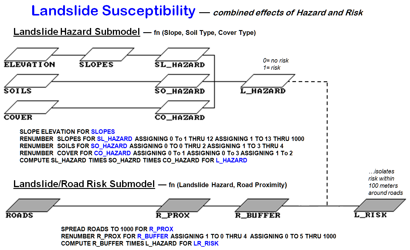
Figure
1. Extends the basic landslide susceptibility model to isolate hazards
around roads (simple proximity “mask”).
The top
portion of figure 1 shows the flowchart and commands for the basic binary landslide
model. The lower portion identifies a risk extension
the basic model that considers proximity to important features as a risk
indicator. In the flowchart, a map of
proximity to roads (R_PROX) is generated that identifies the distance from
every location to the nearest road.
Increasing map values indicate locations farther from a road. A binary map of buffers around roads
(R_BUFFERS) is created by renumbering the distance values near roads to 1 and
far from roads to 0. By multiplying this
“masking" map by the landslide susceptibility map (L_HAZARD), the
landslide threat is isolated for just the areas around roads (risk).
A
further extension to the model involves variable-width buffers as a function of
slope (figure 2). The logic in that refinement is that in steep areas the
buffer width increases as a landslide poses a greater threat. The threat diminishes in gently sloped areas,
so the buffer width contracts. The
weighted buffer extension calibrates the slope map into an impedance map
(FRICTION), which guides the proximity measurement.
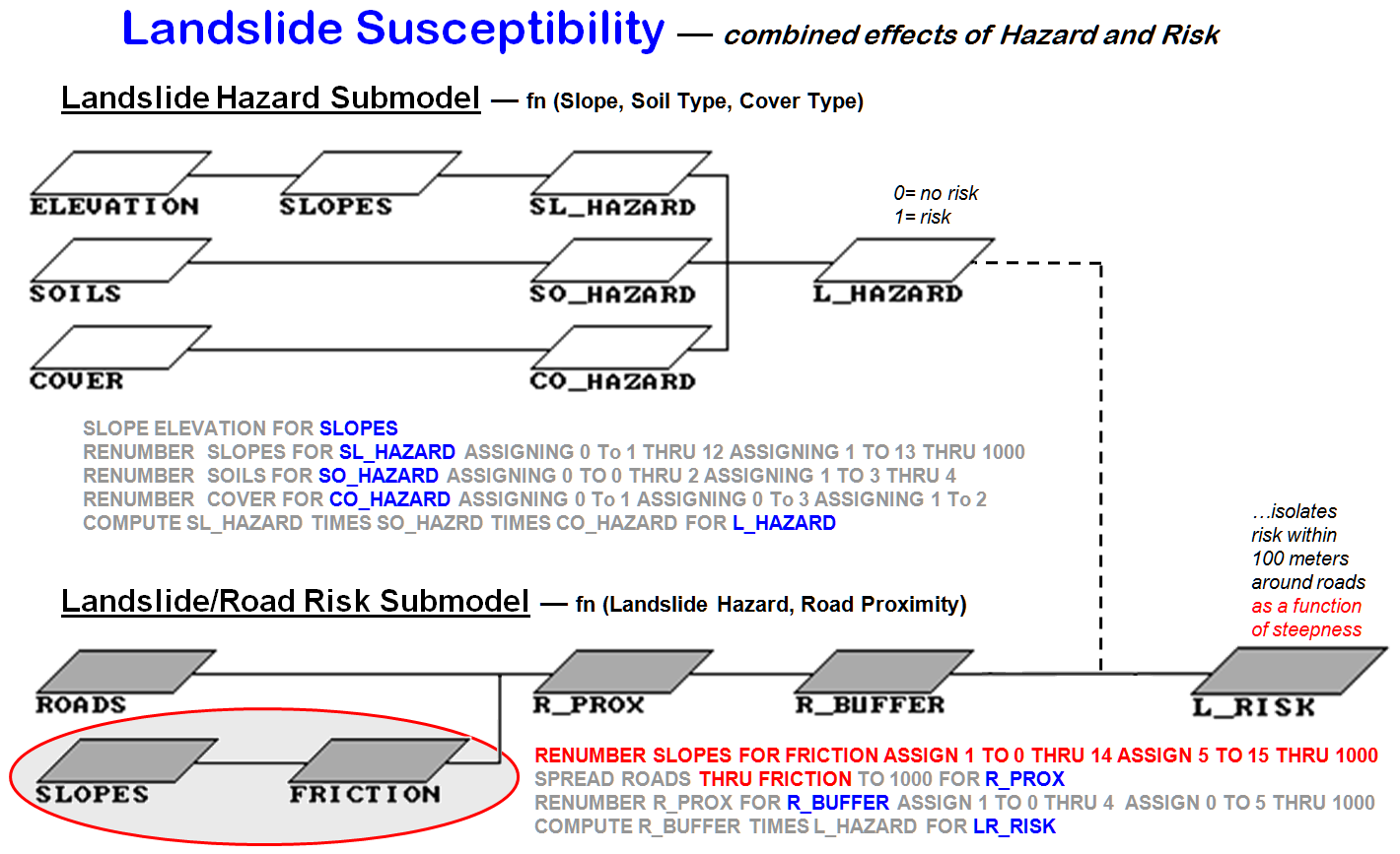
Figure 2. Weighted buffer extension
to the basic landslide susceptibility model.
As the
computer calculates distance in steep areas (low impedance), it assigns larger
effective distance values for a given geographic step than it does in gently
sloped areas (high impedance). That
results in an effective proximity map (R_WPROX), with increasing values
indicating locations that are effectively farther away from the road. The buffer map from these data is radically
different from the simple buffer in the previous model extension.
Instead
of a constant geographic reach around the roads, the effective buffer varies in
width, as a function of slope, throughout the map area. As before, the buffer can be used as a binary
mask to isolate the hazards within the variable reach of the roads.
That
iterative refinement characterizes a typical approach to GIS modeling— from
simple to increasingly complex. Most
applications first mimic manual map analysis procedures and are then extended
to include more advanced spatial analysis tools. For example, a more rigorous map-ematical approach to the previous extension might use a
mathematical function to combine the effective proximity (R_WPROX) with the
relative hazard rating L_HAZARD) to calculate a risk index for each
location.
For
your enjoyment, some additional extensions are suggested below. Can you modify the flowchart to reflect the
changes in model logic? If you have
TMAP, can you develop the additional code?
If you're a malleable undergraduate, you have to if you want to pass the
course. But if you're a professional,
you need not concern yourself with such details. Just ask the l8 year old GIS hacker down the
hall to do your spatial reasoning.
HAZARD
SUBMODEL MODIFICATIONS
-
Consideration of other physical factors,
such as bedrock type, depth to bedrock, faulting, etc.
-
Consideration of disturbance factors,
such as construction cuts and fills
-
Consideration of environmental factors, such
as recent storm frequency, intensity and duration
-
Consideration of seasonal factors, such
as freezing and thawing cycles in early spring
-
Consideration of historical landslide
data earthquake frequency
RISK
SUBMODEL MODIFICATIONS
-
Consideration of additional important
features, such as public, commercial, and residential structures
-
Extension to differentially weight the
uphill and downhill slopes from a feature to calculate the effective buffer
-
Extension to preferentially weight roads
based on traffic volume, emergency routes, etc.
-
Extension to include an economic
valuation of threatened features and potential resource loss
Evaluating Map-ematical Relationships
(GeoWorld, February 1996)
As noted
in the two previous sections, GIS applications come in a variety of forms. The differences aren't as much in the
ingredients (maps) or the processing steps (command macros) as in the conceptual
fabric of the process. In the extensions in the evolution of the landslide
susceptibility, differences in the model approaches can arise through model logic
and/or model expression. A Simple Binary susceptibility model (only
two states of either Yes or No) is radically different from a Weighted Rating model using a weighted
average of relative susceptibility indices.
In mathematical terms, the rating model is more robust, because it
provides a continuum of system responses.
Also, it provides a foothold to extend the model even further.
There
are two basic types of GIS models: cartographic and spatial. In short, a cartographic model focuses on automating manual map analysis
techniques and reasoning, and a spatial
model focuses on expressing mathematical relationships. In the landslide example, the logical
combination and the binary map algebra solutions are obviously cartographic
models. Both could be manually solved
using file cabinets and transparent overlays-tedious, but feasible for the
infinitely patient. The
weighted average rating model, however, smacks of down and dirty map-ematics and looks like a candidate spatial model. But is it?
As with
most dichotomous classifications there is a gray area of overlap between
cartographic and spatial model extremes.
If the weights used in rating model averaging are merely guess-timates, then the application lacks all of the rights,
privileges, and responsibilities of an exalted spatial model. The model may be mathematically expressed,
but the logic isn't mathematically derived, or empirically verified. In short, "Where's the
science?"
One way
to infuse a sense of science is to perform some data mining. That involves locating a lot of areas with
previous landslides, then pushing a predictive statistical technique through a
stack of potential driving variable maps.
For example, you might run a regression on landslide occurrence
(dependent mapped variable) with %slope, %clay, %silt,
and %"cover (independent mapped variables). If you get a good fit, then substitute the
regression equation for the weighted average in the rating model. That approach is at the threshold of science,
but it presumes your database contains just the right set of maps over a large
area. An alternative is to launch a
series of "controlled" experiments under various conditions (%slope,
soil composition, cover density, etc.) and derive a mathematical model through
experiment. That's real science, but it
consumes a lot of time, money, and energy.
A
potential shortcut involves reviewing the scientific literature for an existing
mathematical model and using it. That
approach is used in figure 1, a map-ematical
evaluation of the Revised Universal Soil Loss Equation (RUSLE)—
kind of like landslides from a bug's perspective. The expected soil loss per acre from an area,
such as a farmer's field, is determined from the product of six factors: the
rainfall, the erodibility of the soil, the length and steepness (gradient) of
the ground slope, the crop grown in the soil, and the land practices used. The RUSLE equation and its variable
definitions are shown in figure 1. The
many possible numerical values for each factor require extensive knowledge and
preparation. However, a soil
conservationist normally works in a small area, such as a single county, and
often needs only one or two rainfall factors (R), values for only a few soils
(K), and only a few cropping/practices systems (C and P). The remaining terrain data (L and S) are
tabulated for individual fields.
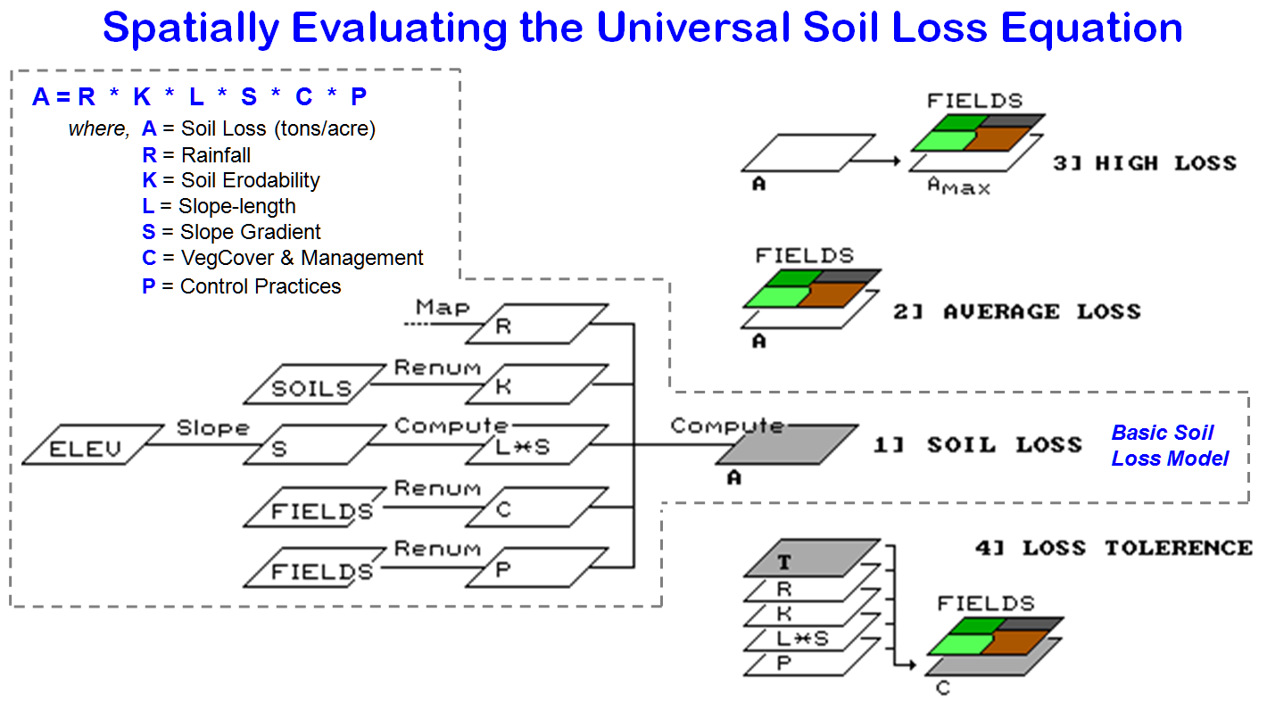
Figure
1. Basic GIS model of the Revised Universal Soil
Loss Equation and extensions.
The
RUSLE model can be evaluated two ways: aggregated or disaggregated. An aggregated
model uses a spatial database management system (DBMS) to store the six factors
for each field, and then solves the equation through a database query. A map of predicted soil loss by individual
field can be displayed, and the total loss for an entire watershed can be
calculated by summing each of the constituent field losses (loss per acre
multiplied by number of acres). That
RUSLE implementation provides several advancements, such as geo-query access,
automated acreage calculations, and graphic display, over the current
procedures.
However,
it also raises serious questions. Many
fields don't fit the assumptions of an aggregated model. Field boundaries reflect ownership rather
than uniformly distributed RUSLE variables.
Just ask any farmer about field variability (particularly if their
field's predicted soil loss puts them out of compliance). A field might have two or more soils, and it
might be steep at one end and flat on the other. Such spatial variation is known to the GIS
(e.g., soil and slope maps), but not used by the aggregated model. A disaggregated
model breaks an analysis unit (farmer's field in this case) into spatially
representative subunits. The equation is
evaluated for each of the subunits, and then combined for the parent
field.
In a
vector system, the subunits are derived by overlaying maps of the six RUSLE
factors, independent of ownership boundaries.
In a raster system, each cell in the analysis grid serves as a
subunit. The equation is evaluated for
each "composite polyglet" or "grid
cell," then weight-averaged by area for the entire field. If a field contains three different factor
conditions, the predicted soil loss proportionally reflects each subunit's
contribution. The aggregated approach
requires the soil conservationist to fudge the parameters for each of the
conditions into generally representative values, and then run the equation for
the whole field. Also, the aggregated
approach loses spatial guidance for the actual water drainage— a field might
drain into two or more streams in different proportions.
Figure
1 shows several extensions to the disaggregated model. Inset 1
depicts the basic spatial computations for soil loss. Inset 2
uses field boundaries to calculate the average soil loss for each field based
on its subunits. Inset 3 provides additional information not available with the
aggregated approach. Areas of high soil
loss (AMAX) are isolated from the overall soil map (A), and then combined with
the FIELDS map to locate areas out of compliance. That directs the farmer's attention to
portions of the field which might require different management action.
Inset 4
enables the farmer to reverse calculate the RUSLE equation. In this case, a soil loss tolerance (T) is
established for an area, such as a watershed, and then the combinations of soil
loss factors meeting the standard are derived.
Because the climatic and physiographic factors of R, K, L, and S are
beyond a farmer's control, attention is focused on vegetation cover (C) and
control practices (P). In short, the
approach generates a map of the set of crop and farming practices that keep the
field within soil loss compliance— good information for decision making.
OK,
what's wrong with the disaggregated approach?
Two things: our databases and our science. For example, our digital maps of elevation
may be too coarse to capture the subtle tilts and turns that water
follows. And the science behind the
RUSLE equation may be too coarse (modeling scale) to be applied to quarter-acre
polyglets or cells.
These limitations, however, tell us what we need to d0— improve our data
and redirect our science. From that
perspective, GIS is more of a revolution in spatial reasoning than an evolution
of current practice into a graphical form.
________________________
Author's Note: Let me apologize for this brief treatise on an
extremely technical subject. How water
cascades over a surface, or penetrates and loosens the ground, is directed by
microscopic processes. The application
of GIS (or any other expansive mode) by its nature muddles the truth. The case studies presented are intended to
illustrate various GIS modeling approaches and stimulate discussion about
alternatives.
(Back
to the Table of Contents)