|
Topic 7 – Organizing the
Map Analysis Toolbox |
Spatial Reasoning
book |
What
Does Your Computer Really Think of Your Map? — discusses
Spatial Topology through the differences among Graphics Packages, Mapping
Software, Spatial Database Management Systems, and GIS Analysis/Modeling
Approaches
Classifying the Analytical
Capabilities of GIS — discusses the differences and similarities in
the Berry and Tomlin map analysis classification schemes
Resolving
Map Detail
— discusses
the four basic types Map Resolution (Spatial, Minimum Mapping, Thematic and
Temporal) that define the level of detail in a digital map as dramatically
different from the traditional concept of Map Scale
<Click here> for a printer-friendly version of this topic
(.pdf).
(Back to the Table of Contents)
______________________________
What Does
Your Computer Really Think of Your Map?
(GeoWorld, November 1994)
To a
human, a map is an image composed of colorful symbols. When you see a couple of red lines cross,
your graphical intuition says, “a road intersection." When two blue lines combine into one, you
think, "fork in a stream." As your eyes wander across a soil map, you
easily grasp which soil unit is adjacent to which. Such truths are self-evident.
But
that's not the case for a computer-compatible map. To the computer, a map is simply an organized
set of numbers— no colored lines, no patterned globs. All of the relationships among map features
must be captured in the number set, or the computer can't "see" the
map. The term spatial topology describes the concept of this linkage, and can be
thought of as information added to the pile of map coordinates.
Take a
look at the map of the United States shown in figure 1. It's easy for you to detect the
characteristic bumps for Florida, New England, and Texas. But the computer only sees thousands of
"on-and-off" dots. If an
individual dot is on, the computer assigns the appropriate color; it's totally
unaware, however, of any patterns formed.
This myopic rendering is characteristic of a graphics package. They're
great for painting maps, but fail to offer the spatial topology needed for map
analysis. A graphics package can't tell
the difference between a map and the graphical rendering of a rose petal-both
are just a pile of unrelated dots.
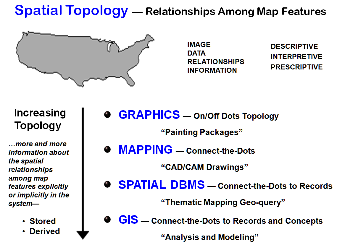
Figure
1. Spatial topology indicates the degree to
which relationships among map features are known to the computer.
A mapping package is a bit more
sophisticated, as it has "connect-the-dots" topology that outlines a
distinct object. The data structure
divides the set of all coordinates into piles, with a separate group for each
distinct feature. One approach uses a "header"
to identify the number of following coordinates that define the feature. If a point feature is indicated, only a pair
of coordinates will follow. For a line
feature, the header is followed by a string of coordinates connected
sequentially. A polygonal feature marks
a string of connected coordinates that closes on itself. That's the basic structure for an AutoCAD .DXF
file— whether it's a blueprint for a sewage plant or a map of the world.
A spatial database management system
extends this ca>based structure to a "connect-the-dots-to-records"
relationship. These packages link a
CAD-like database, identifying the location of each map feature (spatial
record), to another database containing information about each of the features
(thematic records). The linkage is made
through a common identification number (ID#) for each feature contained in the
spatial and thematic datasets.
If you
want to know which countries have a population greater than 200 million, the
computer searches the appropriate field in the thematic database (thematic
entry), then uses the ID#s to find the appropriate coordinates to draw each
country that satisfies the query.
Similarly, a user can "mouse-click" on a country (spatial
entry) and pop up a particular record, a summary of records, or all
informational records from the thematic database. A spatial database management system isn't
your typical dumb map. The computer
knows a lot about each map feature (maybe more than you do, or at least more
than you can remember).
However,
there are still several gaps in the computer's full understanding of the
map. To be a GIS, the computer needs
"connect-the-dots-to-records-and-concepts" topology. It needs to keep track of the relationships
among connecting and adjacent map features. For example, the common boundary
(termed an arc) between two polygons
includes its "from and to" starting points
(termed nodes) and the "left and
right" polygons it divides. A
network of linear features, such as roads or streams, notes which arcs connect
to each other and the cost of traversing each arc in either direction. All this extra baggage of spatial topology
does nothing to enhance the graphical rendering of a map; it merely gets in the
way.
We go
to all this trouble, however, because the computer can’t find its way around on
a non-topological map. A CAD-based road
map might look good to you, but your computer sees a disorganized jumble of
line segments. To determine an optimal
path (or any path for that matter), the computer must have the connections you
see stored in the dataset it manipulates.
To determine the visual connectivity from one location to another, the
computer needs to know the relative intervening elevations. To determine cover type diversity, it needs
to quickly identify adjoining cover types around a location.
Each
GIS package strikes a balance between stored and derived spatial topology. Vector
systems tend to store a lot of their topology in the spatial tables
linked to the thematic database. A
simple "hit to disk" tells the computer the adjacent soil polygon or
the next line segment along a road. Raster systems tend to derive
their topology "on the fly', while processing the data. Finding an adjacent polygon or the next road
cell involves a search of eight neighboring cells. In both vector and raster systems, intricate
spatial relationships (e.g., point in polygon, intersecting lines, or effective
buffers) are derived using the basic analytics in the GIS tool kit. Complex relationships involve spatial models
containing several lines of code.
A GIS
needs full spatial topology (connect the dots to records and concepts) to
perform spatial analysis. As more
information about the relationships among map features is bundled into the data
structure or GIS tool set, the GIS can perform more work for you. If the system is kept in the dark, it can
only draw a map-a simple picture of its database.
Classifying the Analytical Capabilities of GIS
(GeoWorld, March 1996)
“It’s like nailing jelly to a tree.”
Classifying
GIS analytical operations is a bit sticky.
Tremendous inroads have been made toward a common understanding of data
exchange formats, data structures, and even data content standards. However, agreement on a common, conceptual
structure for GIS functionality remains elusive.
In
part, that's due to the diverse disciplines claiming title to GIS and to their
varied perspectives on what it should do.
Coupled with these user differences is the vendor community's desire for
product differentiation. The result is a
quagmire in communicating GIS capabilities and freely exchanging application
models.
Most
GIS textbooks identify an essential set of GIS components as data input
(encode), data management (store), manipulation/analysis (process), and product
output (display). Discussions on the
manipulation/analysis component tend to sort GIS operations into two broad
categories: thematic and spatial. Thematic operations focus on what,
or the attributes that describe map features.
They involve processes such as data reclassification, aggregation,
query, and conditional statements. For
example, locating all of the management parcels (map features) containing Cohassett soil and Douglas fir trees (“what” attributes)
involves a simple query to the management database, followed by a map display
of the results.
Spatial operations focus
on where, or location, and involve processing such as geometric
translations, measurement, coincidence, and spatial statistics. These operations go beyond repackaging
descriptive map data to creating entirely new spatial information and/or map
features. For example, you could overlay
a map of management parcels with a map of terrain steepness to derive an entirely
new map identifying the average slope for each of the management parcels. As a result, you have new information
(average slope) that didn't previously exist in the database. Or, the overlay could generate a new map with
the management parcels partitioned into a subset of new map features based on
the relative terrain steepness within the parcel.
At
first, the distinction between thematic and spatial operations might seem
trivial— merely semantics among the academics.
However, the distinction is a major determinant of current GIS
applications. Thematic operations
reflect well-established database procedures that follow standard Structured
Query Language (SQL) protocol. As a
result, these applications have a large following of users within the greater
computer community.
Spatial
operations, however, present new concepts and foreign procedures. To a confused GlS-neophyte,
there appear to be as many organizational schemes for spatial operations as
there are GIS products and textbooks.
However, there are a few common threads among the different
taxonomies. First, they all
differentiate spatial analysis from “house-keeping" (encoding and storage)
and “visualization” (query and display).
Second, they all agree that spatial analysis implies creating new mapped
data— either new feature characteristics or new spatial partitioning.
The
differences in organizational schemes tend to arise from the taxonomical
structure itself-primarily a dichotomy between the developer and user
camps. Developer-oriented schemes group
the various spatial operations by how they work. This approach is well-suited for GIS
developers, programmers, and specialists, because it rerates to the algorithmic
approaches ingrained in GIS processing.
For example, Tomlin’s comprehensive book on spatial analysis identifies
three “functional groups” based on how the computer algorithm obtains mapped
data for processing (see Author’s Note):
1. Local functions involve single individual locations.
2. Focal and incremental functions
involve values of immediate or extended neighborhoods.
3. Zonal functions involve entire or
partial zones, or regions.
User-oriented
schemes, however, focus on input and output products. The approach is appropriate for general GIS
users because it “relates to familiar manual map processing procedures.” My favorite identifies four functional groups
(see Author’s Notes):
1. Reclassification
operations assign a new value to each map feature on a single
map based on the feature's position, initial value, size, shape, or
contiguity (clumps).
2. Overlay
operations assign new values summarizing
the coincidence of map features from two or more maps based on a
point-by-point, region-wide, or map-wide basis.
3. Distance measurement
operations assigns map values based on
simple or weighted connections among map features including distance,
proximity, movement, and connectivity (optimal paths, line-of-sight, and
narrowness).
4. Neighborhood
operations assign map values that
summarize conditions within the vicinity of map locations (roving window)
based on surface configuration or statistical summary.
From a
developer's perspective, calculating "average slope" for each
management parcel is a zonal operation (summary of slope data within each
parcel), whereas the "partitioning" of individual parcel/slope
subdivisions is a local operation (intersecting vector lines or raster
cells). From a user's perspective both
are simply overlay operations that involve the coincidence of two maps. The distinctions arise because the developer
relates to the differences in the two algorithms, while the user relates to
manually superimposing the two maps on a light table.
A third
perspective, “application-orientation,” also is used to organize spatial
operations. For example, Environmental Systems Research Institute, Inc.'s GRID
cell-based modeling toolkit contains more than 200 operations organized into 20
functional groups. The scheme draws from
focal and zonal functions (reclassification and distance functions), and
identifies application-specific groups to include geometric transformation,
statistical, surface and shape analysis functions. Most of the groups, however, distinguish
among map-ematical operations to include arithmetic,
Boolean, relational, bitwise, combinatorial, logical, accumulative, assignment,
trigonometric, exponential, and logarithmic.
Two
things should be apparent: (1) we aren't clear about what GIS can do, and (2)
we desperately need to be more clear. Before GIS can become a useful button on
everyone's computer, there needs to be a level of consistency in processing
structure that approaches what's being established in data structures. Without such consistency, we might be able to
exchange data, but our spatial reasoning with the data will be fragmented and
incomplete-a GIS Tower of Babel. Of
course, data considerations aren't nailed down either. But that's another
story.
Resolving
Map Detail
(GeoWorld, December 1994)
What determines
a map's accuracy? There are a lot of
factors, but some important ones hinge on the concept of resolution. That's not a
reference to the determination or tenacity of the cartographer, but a measure
of the “level of detail” captured in a map.
If a map captures more detail than another map, it has a higher (or
finer) resolution.
In one
sense, resolution can be related to map scale.
We all know that more detail is seen in a map at 1:24,000 (large/local
scale) than one of the same area at 1:2,000,000 (small/global scale). The effect is that we have only a few inches
of space on a sheet of paper, and if each inch on the paper represents
24,000,000 inches on the ground (2,000,000 feet nearly 400 miles), there isn't
much room for details— hence, low resolution.
But
scale only mathematically relates map measurements to actual ground
distances. It doesn't fully account for
the informational scale of a map. Minimum mapping resolution (MMR) notes
the "level of spatial aggregation," which can be thought of as the
smallest area that can be circled and called one thing. For example, the MMR for a l:24,000 vegetation map is typically less than five
acres. Sure you can discern a single
tree, but would you circle it and call it a timber stand? What's it take-two trees, 10 trees ...?
The MMR
for a l : 24,000 soils map is often six to 20 acres,
with abundant disclaimers about possible "pockets" of other soils
(globs of different soils smaller than the MMR). This informational scale is left to the
discretion of the photo interpreter or field technician— largely a function of
experience, the pen's width, air photo scale, and the discernability
and homogeneity of the forest and soil units.
Another
scale-related consideration is spatial
resolution, identifying "the smallest addressable unit of space"
used in delineating map features. In a
vector system, the smallest addressable unit is the implied line segment
connecting two points. If a point
feature is denoted, the length of the line segment is zero, and the spatial
resolution is at coordinate accuracy of the reference grid + digitizing
error.
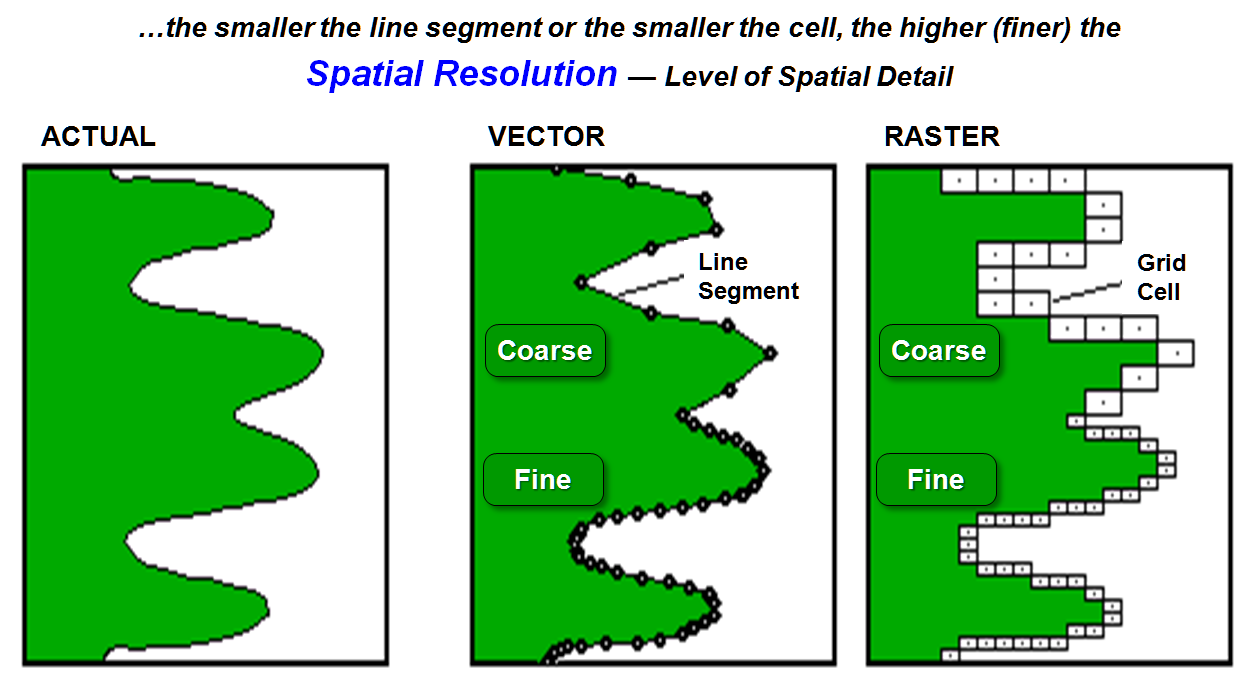
Figure
1.
Spatial resolution identifies the smallest addressable unit of space. It's the line segment in a vector system, and
it's the cell size in a raster system.
As
shown in figure 1, the spatial resolution of an arc is a function of the
spacing of the digitized points— the closer the points, the higher the spatial
resolution (especially on curved segments).
A measure of the spatial resolution for a line involves the ratio of
deflections in the X and Y directions to line segment length.
The
spatial resolution for a raster system is simply the size of cell implied by
the analysis grid— the smaller the cell, the higher the spatial resolution (see
figure 1). Point features, such as a
spring on a water map, are assumed to be contained in a single cell, with the
minimal positional accuracy of one-half the diagonal of the cell.
Feature
size and positioning aren't the only determinants of map detail. Thematic
resolution identifies the smallest classification grouping of a map theme
(see figure 2). In some applications, a
simple forest/non-forest map might provide a sufficient description of
vegetative cover. For years, this coarse
classification has appeared as green on U.S. Geological Survey topographic
sheets. Resource managers require a higher
thematic resolution, however, and expand the classification scheme to include
forest species, age and stocking level.
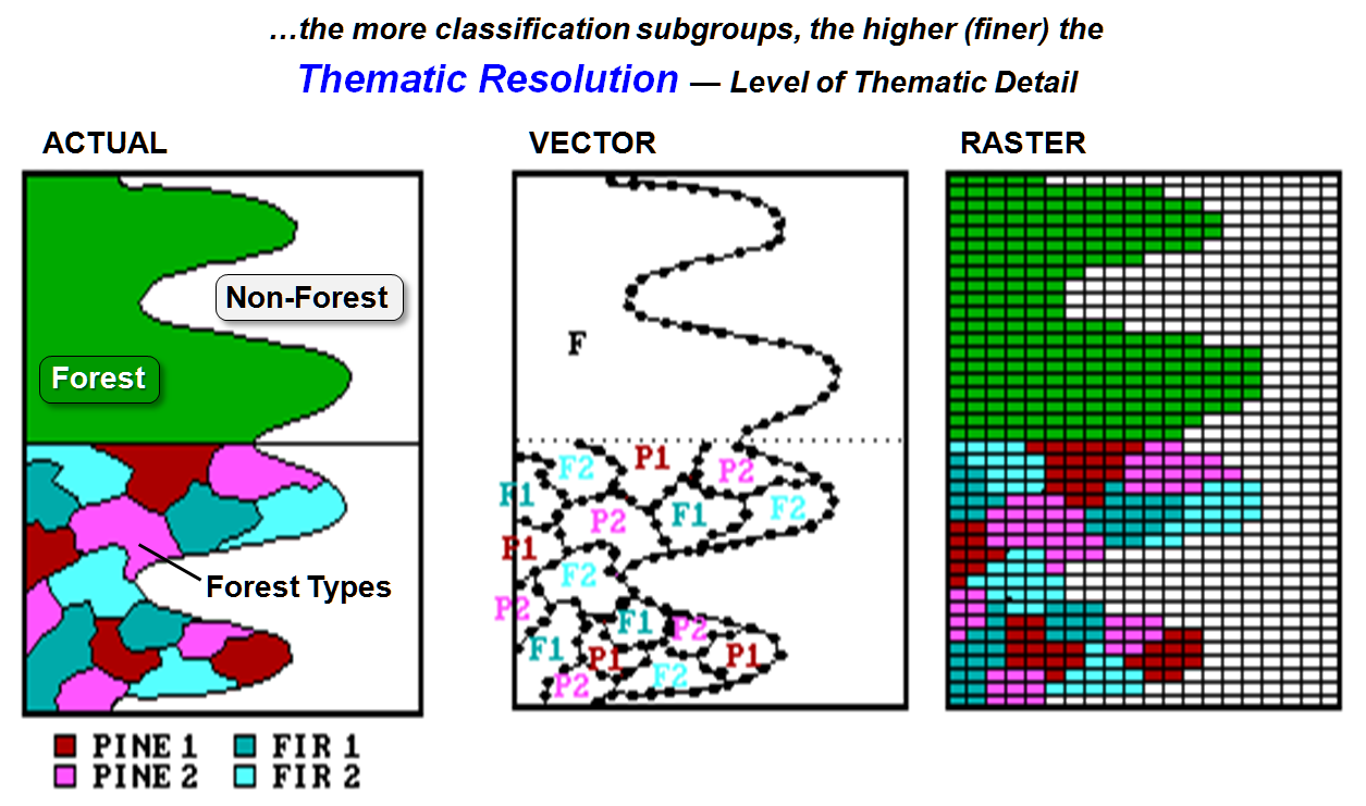
Figure
2. Thematic
resolution identifies the smallest classification grouping of a map theme.
Another
dimension of resolution, termed temporal
resolution, identifies the frequency of map update. For example, a county planner might be
content with a land-use map that's updated every couple of years. The farm agent for the county, however, needs
the agricultural land-use theme broken into farm production classes (finer
thematic resolution), and these areas need to be updated a couple of times each
year (finer temporal resolution).
The
concept of informational scale is important in GIS database design. A corporate database requires consistency
among its mapped data, or at least specification and translation procedures to track
and adjust for inconsistencies. That's a
far cry from the traditional plethora of personal paper maps.
For
8,000 years, geographic scale has been the de facto indicator of map
detail. But times have changed, and
measures of mapping, spatial resolution, thematic resolution and temporal
resolution should be integral parts of the modern map's legend and processing
procedures. Just keep in mind, the next
time your GIS slams a few maps together, that simply translating to the same
geographic scale and projection doesn't ensure consistent informational
scales. And we all know what happens
when you mix scales (ahhhhha!).
_______________________