|
Topic 5 –
Structuring GIS Modeling Approaches |
GIS
Modeling book |
Mixing
It up in GIS Modeling’s Kitchen — an overview of map
analysis and GIS modeling considerations
How
to Determine Exactly “Where Is What” — discusses the
levels of precision (correct placement) and accuracy (correct characterization)
Getting
the Numbers Right — describes a classification scheme for map
analysis operations based on how map values are retrieved for processing
(Local, Focal, Zonal)
Putting GIS Modeling Concepts in Their Place — develops a typology of GIS modeling
types and characteristics
A Suitable Framework for GIS Modeling — describes a framework for
suitability modeling based on a flowchart of model logic
Further Reading
— two additional sections
<Click here>
for a printer-friendly version of this
topic (.pdf).
(Back to the Table of Contents)
______________________________
Mixing It up in GIS Modeling’s Kitchen
(GeoWorld, May 2013)
The modern “geotechnology
recipe” is one part data, one part analysis and a dash of colorful
rendering. That’s a far cry from the
historical mapping recipe of basically all data with a generous ladling of
cartography. Today’s maps are less
renderings of “precise placement of physical features for navigation and
record-keeping” (meat and potatoes) than they are interactive “interpretations
of spatial relationships for understanding and decision-making” (haute
cuisine).
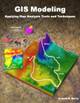
Figure 1 carries this
cheesy cooking analogy a few steps further.
The left portion relates our modern food chain to levels of mapped data
organization from mouthfuls of map values to data warehouses. The center and right side of the figure ties
these data (ingredients) to the GIS modeling process (preparation and cooking)
and display (garnishing and presentation).
A map stack of
geo-registered map layers is analogous to a pantry that contains the necessary
ingredients (map layers) for preparing a meal (application). The meal can range from Pop-Tart à la mode
to the classic French coq
au vin or Spain’s paella with their increasing complexity and varied
ingredients, but a recipe all the same.
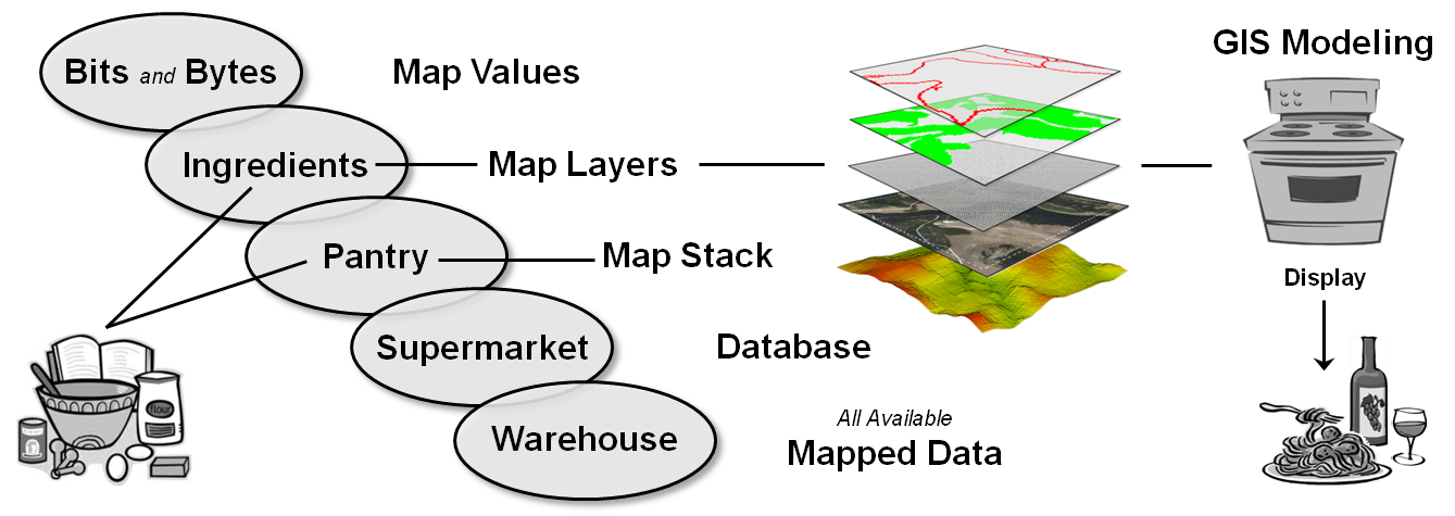
Figure 1. The levels of mapped data organization are
analogous to our modern food chain.
GIS Modeling is sort of
like that but serves as food for quantitative thought about the spatial
relationships and patterns around us. To
extend the cooking analogy, the rephrasing of an old saying seems appropriate—
“Bits and bytes may break my bones, but inaccurate modeling will surely poison
me.” This suggests that while bad data
can certainly be a problem, ham-fisted processing of perfect data can spoil an
application just as easily.
For example, a protective
“simple distance buffer” of a fixed distance is routinely applied around
spawning streams ignoring relative erodibility of intervening
terrain/soil/vegetation conditions. The
result is an ineffective buffer that continues to rain-down dirt balls that
choke the fish in highly erodible palaces and starve-out timber harvesting in
places of low erodibility. In
this case, the simple buffer is a meager “rice-cake-like” solution that
propagates at megahertz speed across the mapping landscape helping neither the
fish nor the logger. A more elaborate
recipe involving a “variable-width buffer” is needed, but it is rarely
employed.
GIS tends to focus a
great deal on spatial data structure, formats, characteristics, query and
visualization, but less on the analytical processing that “cooks” the data
(meant in the most positive way). So
what are the fundamental considerations in GIS models and modeling? How does it relate to traditional modeling?
At the highest conceptual
level, GIS modeling has two important characteristics—processing structure and
elemental approaches. The center portion
of figure 2 depicts the underlying Processing Structure for all
quantitative data analysis as a progression from fundamental operations
to generalized techniques to key sub-models and finally to full
application models.
This traditional
mathematical structure uses sequential processing of basic math/stat operations
to perform a wide variety of complex analyses.
By controlling the order in which the operations are executed on
variables, and using common storage of intermediate results, a robust and
universal mathematical processing structure is developed.
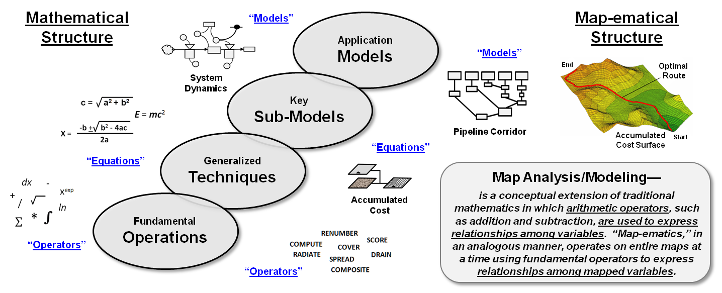
Figure 2. The
"map-ematical structure" processes entire map layers at a time using
fundamental operators to express relationships among mapped variables in a
manner analogous to our traditional mathematical structure.
The
"map-ematical" structure is similar to traditional algebra in which
primitive operations, such as addition, subtraction, and exponentiation, are
logically sequenced for specified variables to form equations and models. However in map algebra 1) the variables
represent entire maps consisting of geo-registered sets of map values, and 2)
the set of traditional math/stat operations are extended to simultaneously
evaluate the spatial and numeric distributions of mapped data.
Each processing step is
accomplished by requiring—
-
retrieval
of one or more map layers from the map stack,
-
manipulation
of that mapped data by an appropriate math/stat operation,
-
creation
of an intermediate map layer whose map values are derived as a result of that
manipulation, and
-
storage
of that new map layer back into the map stack for subsequent processing.
The
cyclical nature of the retrieval-manipulation-creation-storage processing structure
is analogous to the evaluation of “nested parentheticals” in traditional
algebra. The logical sequencing of map
analysis operations on a set of map layers forms a spatial model of specified
application. As with traditional
algebra, fundamental techniques involving several primitive operations can be
identified that are applicable to numerous situations.
The
use of these primitive map analysis operations in a generalized modeling
context accommodates a variety of analyses in a common, flexible and intuitive
manner. Also it provides a framework for
understanding the principles of map analysis that stimulates the development of
new techniques, procedures and applications (see author’s note 1).
The
Elemental
Approaches
utilized in map analysis and GIS modeling also are rooted in traditional
mathematics and take on two dimensions— Atomistic/Analysis versus
Holistic/Synthesis.
The Atomistic/Analysis
approach to GIS modeling can be thought of as “separating a whole into
constituent elements” to investigate and discover spatial relationships
within a system (figure 3). This
“Reductionist’s approach” is favored by western science which breaks down
complex problems into simpler pieces which can then be analyzed
individually.
Figure 3. The two Elemental Approaches utilized in
map analysis and GIS Modeling.
The Holistic/Synthesis
approach, in contrast, can be thought of as “combining constituent elements
into a whole” in a manner that emphasizes the organic or functional
relationships between the parts and the whole.
This “Interactionist’s approach” is often associated with eastern
philosophy of seeing the world as an integrated whole rather than a dissociated
collection of parts.
So what does all this
have to do with map analysis and GIS modeling?
It is uniquely positioned to change how quantitative analysis is applied
to complex real-world problems. First, it
can be used account for the spatial distribution as well as the numerical
distribution inherent in most data sets.
Secondly, it can be used in the atomistic analysis of spatial systems to
uncover relationships among perceived driving to variables of a system. Thirdly, it can be used in holistic synthesis
to model changes in systems as the driving variables are altered or generate
entirely new solutions.
In a sense, map analysis
and modeling are like chemistry. A great
deal of science is used to break down compounds into their elements and study
the interactions—atomistic/analysis. Conversely, a great deal of innovation is
used to assemble the elements into new compounds— holistic/synthesis. The combined results are repackaged into
entirely new things from food additives to cancer cures.
Map analysis and GIS
modeling operate in an analogous manner.
They use many of the same map-ematical operations to first analyze and
then to synthesize map variables into spatial solutions from navigating to a
new restaurant to locating a pipeline corridor that considers a variety of
stakeholder perspectives. While
dictionaries define analysis and synthesis as opposites, it is important to
note that in geotechnology, analysis without synthesis is almost worthless …and
that the converse is just as true.
_____________________________
Author’s Notes: 1) see “SpatialSTEM – Seminar, Workshop and
Teaching Materials for Understanding Grid-based Map Analysis” posted at www.innovativegis.com/Basis/Courses/SpatialSTEM/. 2) For more on GIS models and modeling, see
the Beyond Mapping Compilation Series, book II, Topic 5, “A Framework for GIS
Modeling” posted at www.innovativegis.com/basis/.
How to
Determine Exactly “Where Is What”
(GeoWorld, February 2008)
The Wikipedia
defines Accuracy as “the
degree of veracity” (exactness) while Precision
as “the degree of reproducibility” (repeatable). It uses an archery target as an analogy to
explain the difference between the two terms where measurements are compared to
arrows shot at the target (left side of figure 1). Accuracy describes the closeness of arrows to
the bull’s-eye at the target center (actual/correct). Arrows that strike closer to the bulls eye
are considered more accurate.
Precision, on the other hand, relates to the size of the
cluster of several arrows. When the
arrows are grouped tightly together, the cluster is considered precise since
they all strike close to the same spot, if not necessarily near the bull’s-eye. The measurements can be precise, though not
necessarily accurate.
However, it is not possible to reliably achieve
accuracy in individual measurements without precision. If the arrows are not grouped close to one
another, they cannot all be close to the bull’s-eye. While their average position might be an accurate estimation of the
bull’s-eye, the individual arrows are inaccurate.
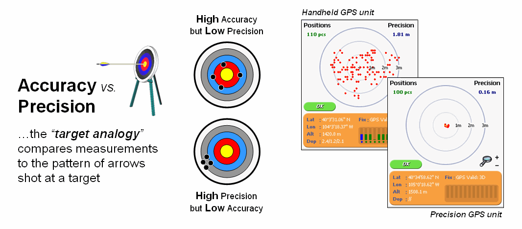
Figure 1. Accuracy refers to “exactness” and Precision
refers to “repeatability” of data.
So what does this academic diatribe have to do with
In
Whereas
Figure 2 illustrates the two-fold consideration of Precise Placement of coordinate
delineation and Accurate Assessment
of attribute descriptor for three photo interpreters. The upper-right portion superimposes three
parcel delineations with Interpreter B outlining considerably more area than
Interpreters A and C—considerable variation in precision. The lower portion of the figure indicates
differences in classification with Interpreter B assigning Ponderosa pine as
the vegetation type—considerable variation in accuracy to the true Cottonwood
vegetation type correctly classified by Interpreters A and C.
Many
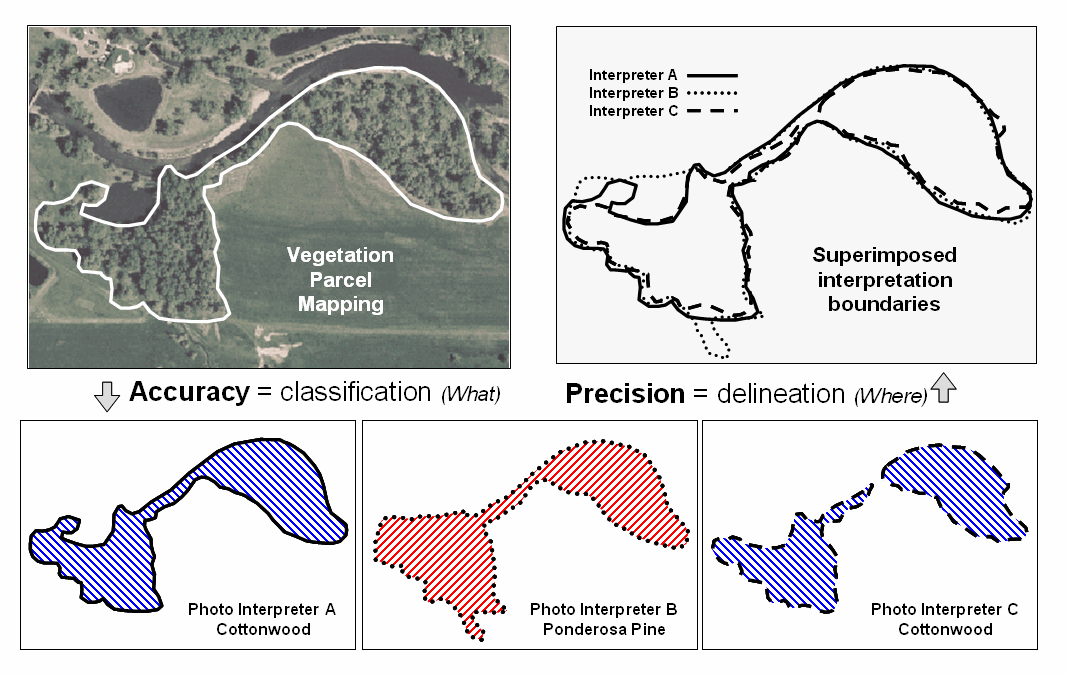
Figure 2. In mapped data, precision refers to placement
whereas accuracy refers to classification.
In addition, our paper map legacy of visualizing maps
frequently degrades precision/accuracy in detailed mapped data. For example, a detailed map of slope values
containing decimal point differences in terrain inclination can be easily
calculated from an elevation surface.
But the detailed continuous spatial data is often aggregated into just a
few discrete categories so humans can easily conceptualize and “see” the information—such
as polygonal areas of gentle, moderate and steep terrain. Another example is the reduction of the high
precision/accuracy inherent in a continuous “proximity to roads” map to that of
a discrete “road buffer” map that simply identifies all locations within a
specified reach.
Further thought suggests an additional consideration of
As you might suspect, different groups have differing
perspectives on the interpretation and relative importance of the routing
criteria. For example, homeowners might
be most concerned about Housing Density and Visual Exposure; environmentalists
most concerned about Road Proximity and Sensitive Areas; and engineers most
concerned about Housing Density and Road Proximity. Executing the model for these differences in
perspective (relative importance of the criteria) resulted in three different
preferred routes.
The lower-left portion of figure 3 shows the spread of
the three individual solutions. One
isn’t more precise/accurate than another, just an expression of a particular
perspective of the solution.
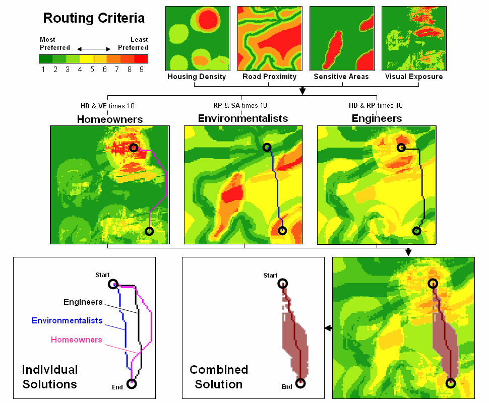
Figure 3. Maps derived by
The lower-right side of the figure suggests yet another
way to represent the solution using the simple average of the three preference
surfaces to identify an overall route and its optimal corridor—sort of
analogous to averaging a series of
The take home from this discussion is that precision and
accuracy is not the same thing and that the terms can take on different
meanings for different types of maps and application settings. There are at least three different levels of
precision/accuracy—1) “Where is Where”
considering just precise placement, 2) “Where
is What” considering placement and classification, and 3) “Where is What, if you assume…”
considering placement, classification and
interpretationà logicà understandingà judgment
ingrained in spatial reasoning.
Before
_____________________________
Author’s Notes: Related
discussion of routing model considerations and procedures is in Topic 8,
Spatial Model Example in the book Map Analysis (Berry, 2007; GeoTec
Media, www.geoplace.com/books/MapAnalysis)
and Topic 19, Routing and Optimal Paths in the online Beyond Mapping
Getting
the Numbers Right
(GeoWorld, May 2007)
The
concept that “maps are numbers first,
pictures later” underlies all GIS processing. However in map analysis, the digital nature
of maps takes on even more importance.
How the map values are 1) retieved and 2) processed establishes a basic
framework for classifying all of the analytical capabilities. In obtaining map values for processing there
are three basic methods— Local, Focal and Zonal (see author’s note).
While
the Local/Focal/Zonal classification scheme is most frequently associated with
grid-based modeling, it applies equally well to vector-based analysis— just
substitute the concept of “polygon, line or point” for that of a grid “cell” as
the smallest addressable unit of space providing the map values for
processing.
Local processing retrieves a map value
for a single map location independent of its surrounding values, then processes
the value to derive and assign a new value to the location (figure 1). For example, an elevation value of 8250
associated with a grid cell location on an existing terrain surface is
retrieved and then the contouring equation of Interval = [Integer((MapValue - ContourBase) / ContourInterval)] =
[int((8250 + 100) / 100)] = 83 is evaluated. The new map value of 83 is stored to indicate
the 83rd 100-foot contour interval (8200-8300 feet) from a sea level
contour base interval of 1 (0 to 100 feet).
The processing is repeated for all map locations and the resultant map
is filed with the other map layers in the stack.
Figure 1. Local operations use point-by-point
processing of map values that occur at each map location.
A
similar operation might multiply the elevation value times 0.3048 [ElevMeters = ElevFeet * 0.3048= 8250 * 0.3048= 2871] to convert
the elevation from feet to meters. In
turn, a generalized atmospheric cooling relationship of 9.78 degC per 1000
meter rise can be applied [(2871 / 1000 *
9.78] to assign a value of 28.08 degC cooler than sea level air (termed Adiabatic Lapse Rate for those who are atmoshperic physics
challenged).
The
lower portion of figure 1 expands the Local processing concept from a single
map layer to a stack of registered map layers. For example, a point-by-point
overlay process might retrieve the elevation, slope, aspect, fuel loading,
weather, and other information from a series of map layers as values used in
calculating wildfire risk for a location.
Note that the processing is still spatially-myopic as it addresses a
single map location at a time (grid cell) but obtains a string of values for that
location before performing a mathematical or statistical process to summarize
the values.
While
the examples might not directly address your application interests, the
assertion that you can add, subtract, multiply, divide and otherwise “crunch
the numbers” ought to alert you to the map-ematical nature of GIS. It suggests a map calculator with all of the
buttons, rights and privileges of your old friendly handheld calculator— except
a map calculator operates on entire map layers composed of thousands upon
thousands of geo-registered map values.
The
underlying “cyclical” structure of Retrieveà Processà Storeà File also
plays upon our traditional math experience.
You enter a number or series of numbers into a calculator, press a
function button and then store the intermediate result (calculator memory or
scrap of paper) to be used as input for subsequent processing. You repeat the cycle over and over to solve a
complex expression or model in a “piece-by-piece” fashion—whether traditional
scaler mathematics or spatial map-ematics.
Figure 2. Focal operations use a vicinity-context to
retrieve map values for summary.
Figure
2 outlines a different class of analytical operators based on how the values
for processing are obtained. Focal processing retrieves a set of map
values within a neighborhood/vicinity around a location. For example a 3x3 window could be used to
identify the nine adjacent elevations at a location, and then apply a slope
function to the data to calculate terrain steepness. The derived slope value is stored for the
location and the process repeated over and over for all other locations in a
project area.
The
concept of a fixed window of neighboring map values can be extended to other
spatial contexts, such as effective distance, optimal paths, viewsheds, visual
exposure and narrowness for defining the influence or “reach” around a map
location. For example, a travel-time map
considering the surrounding street network could be used to identify the total
number of customers within a 10-minute drive.
Or the total number of houses that are visually connected to a location
within a half-mile could be calculated.
Figure 3. Zonal operations use a
separate template map to retrieve map values for summary.
While
Focal processing defines an “effective reach” to retrieve surrounding map
values for processing, Zonal
processing uses a predefine “template” to identify map values for summary
(figure 3). For example, a wildlife
habitat unit might serve as a template map to retrieve slope values from a data
map of terrain steepness. The average of
all of the coincident slope values is computed and then stored for all of the
locations defining the template.
Similarly,
a map of total sales (data map) can be calculated for a set of sales management
districts (template map). The standard
set of statistical summaries is extended to spatial operations such as
contiguity and shape of individual map features.
The
Local/Focal/Zonal organization scheme addresses how analytic operations work
and is particularly appropriate for GIS developers and programmers. The Reclassify/Overlay/Distance/Neighbors
scheme I have used throughout the Beyond Mapping series uses a different
perspective—one based on the information derived and its utility (see, Use a Map-ematical Framework for GIS
Modeling, GeoWorld, March 2004, pg 18-19).
However,
both the “how it works” and “what it is” perspectives agree that
all analytical operations require retrieving and processing numbers within a
cyclical map-ematical environment. The
bottom line being that maps are numbers and map analysis crunches the numbers
in challenging ways well outside our paper-map legacy.
_____________________________
Author’s Note: Local,
Focal and Zonal processing classes were first suggested by Dana Tomin in his
doctoral dissertation “Geographic
Information Systems and Cartographic Modeling” (Yale University, 1980)
and partially used in organizing the Spatial Analyst/Grid modules in ESRI’s
ArcGIS software.
Putting GIS Modeling Concepts in Their Place
(GeoWorld, October 2010)
The vast majority of GIS
applications focus on spatial inventories that keep track of things,
characteristics and conditions on the landscape— mapping and geo-query of Where
is What. Map analysis and GIS
modeling applications, on the other hand, focus on spatial relationships within
and among map layers— Why, So What and What If.
Natural resource fields
have a rich heritage in GIS modeling that tackles a wide range of management
needs from habitat mapping to land use suitability to wildfire risk assessment
to infrastructure routing to economic valuation to policy formulation. But before jumping into a discussion of GIS
analysis and modeling in natural resources it seems prudent to establish basic
concepts and terminology usually reserved for an introductory lecture in a
basic GIS modeling course.
Several years ago I
devoted a couple of Beyond Mapping columns to discussing the various types and
characteristics of GIS models (see Author’s note). Figure 1 outlines this typology with a bit of
reorganization and a few new twists and extensions gained in the ensuing 15
years. The dotted connections in the
figure indicate that the terms are not binary but form transitional gradients,
with most GIS models involving a mixture of the concepts.
Simply stated any model
is a representation of reality in either material form (tangible
representations) or symbolic form (abstract representations). The two general types of models include
structural and relational. Structural
models focus on the composition and construction of tangible things and
come in two basic forms— action involving dynamic movement-based models,
such as a model train along its track and object involving static
entity-based models forming a visual representation of an item, such as an
architect’s blueprint of a building. CAD
and traditional GIS inventory-oriented applications fall under the “object”
model type.
Relational models, on the other hand, focus on the interdependence
and relationships among factors. They
come in two types— functional models based on input/output that track
relationships among variables, such as storm runoff prediction and conceptual
models based on perceptions that incorporate fact interpretation and value
weights, such as suitable wildlife habitat derived by interpreting a stack of
maps describing a landscape.
Fundamentally there are
two types of GIS models—cartographic and spatial. Cartographic models automate manual
techniques that use traditional drafting aids and transparent overlays (i.e.,
McHarg overlay), such as identifying locations of productive soils and gentle
slopes using binary logic expressed as a geo-query. Spatial models express mathematical
and statistical relationships among mapped variables, such as deriving a
surface heat map based on ambient temperature and solar irradiance involving
traditional multivariate concepts of variables, parameters and
relationships.
All GIS models fall under
the general “symbolic --> relational” model types, and because digital maps
are “numbers first, pictures later,” map analysis and GIS modeling are usually
classified as mathematical (or maybe that should be “map-ematical”). The somewhat subtle distinction between
cartographic and spatial models reflects the robustness of the map values and
the richness of the mathematical operations applied.
The general
characteristics that GIS models share with non-spatial models include purpose,
approach, technique and temporal considerations. Purpose identifies a model’s
intent/utility and often involves a descriptive characterization of the
direct interactions of a system to gain insight into its processes, such as a
wildlife population dynamics map generated by simulation of life/death
processes. Or the purpose could be prescriptive
to assess a system’s response to management actions/interpretations, such as
changes in a proposed power line route under different stakeholder’s
calibrations and weights of input map layers.
A model’s Approach
can be empirical or theoretical. An empirical
model is based on the reduction (analysis) of field-collected measurements,
such as a map of soil loss for each watershed for a region generated by
spatially evaluating the empirically derived Universal Soil Loss equation. A theoretical model, on the other
hand, is based on the linkage (synthesis) of proven or postulated relationships
among variables, such as a map of spotted owl habitat based on accepted
theories of owl preferences.
![]()
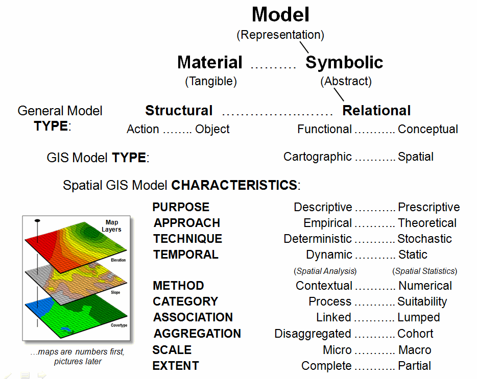
Figure 1. Types and characteristics of GIS models.
Modeling Technique
can be deterministic or stochastic. A deterministic
model uses defined relationships that always results in a single repeatable
solution, such as a wildlife population map based on one model execution using
a single “best” estimate to characterize each variable. A stochastic model uses repeated
simulation of a probabilistic relationship resulting in a range of possible
solutions, such as a wildlife population map based on the average of a series
of model executions.
The Temporal
characteristic refers to how time is treated in a model— dynamic or
static. A dynamic model treats
time as variable and model variables change as a function of time, such as a
map of wildfire spread from an ignition point considering the effect of the
time of day on weather conditions and fuel loading dryness. A static model treats time as a
constant and model variables do not vary over time, such as a map of timber
values based on the current forest inventory and relative access to roads.
The modeling Method,
however, is what most distinguishes GIS models from non-spatial models by
referring to the spatial character of the processing— contextual or
numerical. Contextual methods use
spatial analysis to characterize “contextual relationships” within and among
mapped data layers, such as effective distance, optimal paths, visual
connectivity and micro-terrain analysis.
Numerical methods use spatial statistics to uncover “numerical
relationships” within and among mapped data layers, such as generating a
prediction map of wildfire ignition based regression analysis of historical
fire occurrence and vegetation, terrain and human activity map layers.
Spatial Analysis (contextual spatial relationships) and Spatial
Statistics (numerical spatial relationships) form the “toolboxes” that are
uniquely GIS and are fueling the evolution from descriptive mapping and
“geo-query” searches of existing databases to investigative and prescriptive
map analysis/modeling that address a variety of complex spatial problems— a
movement in user perspective from “recordkeeping” to “solutions.”
The Category
characteristic of GIS models is closely related to the concept of “Relational”
in general modeling but speaks specifically to the type of spatial
relationships and interdependences among map layers. A process-oriented model involves
movement, flows and cycles in the landscape, such as timber harvesting access
considering on- and off-road movement of hauling and harvesting equipment. A suitability-oriented model
characterizes geographic locations in terms of their relative appropriateness
for an intended use.
Model association,
aggregation, scale and extent refer to the geographic nature of how map layers
are defined and related. Association
refers to how locations relate to each other and can be classified as lumped
when the state/condition of each individual location is independent of other
map locations (i.e., point-by-point processing). A linked association, on the other
hand, occurs when the state/condition of each individual location is dependent
on other map locations (i.e., vicinity, neighborhood or regional
processing).
Aggregation describes the grouping of map locations for
processing and is termed disaggregated when a model is executed for each
individual spatial object (usually a grid cell), such as in deriving a map of
predicted biomass based on spatially evaluating a regression equation in which
each input map layer identifies an independent “variable,” each location a
“case,” and each map value a “measurement” as defined in traditional statistics
and mathematical modeling.
Alternatively, cohort
aggregation utilizes groups of spatial objects having similar characteristics,
such as deriving a timber growth map for each management parcel based on a
look-up table of growth for each possible combination of map layers. The model is executed once for each
combination and the solution is applied to all map locations having the same
“cohort” combination.
GIS modeling
characteristics of Scale and Extent retain their traditional
meanings. A micro scale model
contains high resolution (level of detail) of space, time and/or variable
considerations governing system response, such as a 1:1,000 map of a farm with
crops specified for each field and revised each year. A macro scale model contains low
resolution inputs, such as a 1:1,000,000 map of land use with a single category
for agriculture revised every 10 years.
A GIS model’s Extent
is termed complete if it includes the entire set of space, time and/or
variable considerations governing system response, such as a map set of an
entire watershed or river basin. A partial
extent includes subsets of input data that do not completely cover an area of
interest, such as a standard topographic sheet with its artificial boundary
capturing limited portions of several adjoining watersheds.
For those readers who are
still awake, you have endured an introductory academic slap and now possess all
of the rights, privileges and responsibilities of an introductory GIS modeling
expert who is fully licensed to bore your peers and laypersons alike with such
arcane babble. Next month’s discussion
will apply and extend these concepts to model logic, degrees of abstraction,
levels of analysis and processing levels using an example model for assessing
campground suitability.
_____________________________
Author’s Note: If
you have old GW magazines lying about, see “What’s in a Model?” and “Dodge the
GIS Modeling Babble Ground” in the January and February 1995 issues of GIS
World (the earlier less inclusive magazine name for GeoWorld) or visit www.innovativegis.com, and select
Beyond Mapping Compilation Series, Chronological Listing, and scroll down to
the Beyond Mapping II online book of Beyond Mapping columns from October 1993
to August 1996.
A Suitable Framework for GIS Modeling
(GeoWorld, November 2010)
Suitability Modeling is
one of the simplest and most frequently used GIS modeling approaches. These models consider the relative “goodness”
of each map location for a particular use based on a set of criteria.
For example, figure 1
outlines five Criteria considerations for locating a campground: favor
gentle terrain, being near roads and water, with good views of water and
oriented toward the west.
![]()
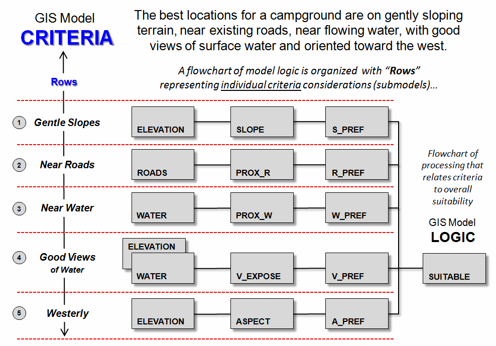
Figure 1. Campground Suitability model logic with
rows indicating criteria.
In the flowchart of the
model’s logic, each consideration is identified as a separate “row.” In essence every map location is graded in
light of its characteristics or conditions in a manner that is analogous to a
professor evaluating a set of exams during a semester. Each spatial consideration (viz. exam) is
independently graded (viz. student answers) with respect to a consistent scale
(viz. an A to an F grade).
Figure 2 identifies Analysis
Levels as “columns” used to evaluate each of the criteria and then combines
them into an overall assessment of campground suitability. Base Maps represent the physical
characteristics used in the evaluations— maps of Elevation, Roads, and Water in
this case. But these “facts” on the
landscape are not in a form that can be used to evaluate campground
suitability.
Derived Maps translate physical descriptions into suitability
contexts. For example, it is not
Elevation per se that affects campground suitability, but the rate and
direction of the change in elevation expressed as Slope and Aspect that
characterize terrain configuration.
Similarly, it is not the presence of roads and water but the relative closeness
to these features that affects the degree of suitability (Prox_R and
Prox_W).
![]()
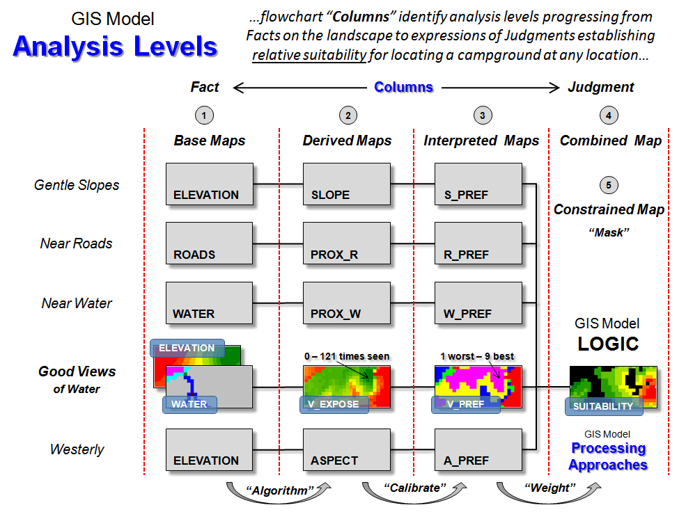
Figure 2.
Flowchart columns represent analysis levels transforming facts into
judgment.
Interpreted Maps identify increasing abstraction from Facts on the
landscape to Judgments within the context of suitability. At this level, derived maps are
interpreted/graded into a relative suitability score, usually on a scale from 1
(least suitable/worst) to 9 (most suitable/best). Using the exam grading analogy, a map
location could be terrible in terms of terms of proximity to roads and water
(viz. a couple of F’s on two of the exams) while quite suitable in terms of
terrain steepness and aspect (viz. A’s on two other exams).
Like a student’s semester
grade, the overall suitability, or Combined Map, for a campground is a
combination of the individual criteria scores.
This is usually accomplished by calculating the simple or
weighted-average of the individual scores.
The result is a single value indicating the overall “relative goodness”
for each map location that in aggregate forms a continuous spatial distribution
of campground suitability for a given project area.
However, some of the
locations might be constrained by legal or practical concerns that preclude
building a campground, such as very close to water or on very steep
terrain. A Constraint Map
eliminates these locations by forcing their overall score to “0”
(unsuitable).
![]()
Figure 3. Processing flow that implements the
Campground Suitability model.
Figure 3 depicts the Processing
Flow as a series of map analysis operations/commands. You are encouraged to follow the flow by
delving into more detail and even complete a hands-on exercise in suitability
modeling (see author’s note)— it ought to be a lot of fun, right?
The logical progression
from physical Facts to suitability Judgments involves four basic Processing
Approaches— Algorithm, Calibrate, Weight, and Mask. For example, consider the goal of “good views
of water.” The derived map of visual
exposure to water (V_Expose) uses an Algorithm that counts the number of
times each location is visually connected to water locations—
RADIATE Water OVER Elevation TO
100 AT 1 Completely FOR V_Expose
…that in this example,
results in values from 0 to 121 times seen.
In turn, the visual exposure map is Calibrated to a relative
suitability scale of 1 (worst) to 9 (best)—
RENUMBER V_Expose ASSIGNING 9 TO 80
THRU 121 ASSIGNING 8 TO 30 THRU 80 ASSIGNING 5 TO 10 THRU 30 ASSIGNING 3 TO 6 THRU 10 ASSIGNING 1 TO 0 THRU 6 FOR V_Pref
The interpreted visual
exposure map and the other interpreted maps are Weighted by using a simple
arithmetic average—
ANALYZE S_PREF TIMES 1 WITH W_PREF TIMES 1
WITH V_Pref TIMES 1 WITH A_PREF TIMES 1 WITH R_PREF TIMES 1 Mean FOR Suitable
Finally, a binary
constraint map (too steep and/or too close to water = 0; else= 1) is used to Mask
unsuitable areas—
COMPUTE Suitable Times Constraints
FOR Suitable_masked
_____________________________
Author’s Note: An
annotated step-by-step description of the Campground Suitability model and
hands-on exercise materials are posed at www.innovativegis.com/basis/Senarios/Campground.htm. Additional discussion of types and approaches
to suitability modeling is in Beyond Mapping Compilation Series book III, Topic
7, “Basic Spatial Modeling Approaches” posted at www.innovativegis.com.
_____________________
Further Online Reading: (Chronological
listing posted at www.innovativegis.com/basis/BeyondMappingSeries/)
Explore the Softer Side of GIS — describes
a Manual GIS (circa 1950) and the relationship between social science
conceptual (January 2008)
Use Spatial Sensitivity Analysis to Assess
Model Response — develops an approach for
assessing the sensitivity of GIS models (August 2009)
(Back
to the Table of Contents)