|
Topic 10 – Future
Directions and Trends |
GIS
Modeling book |
GIS
Innovation Drives Its Evolution — discusses the cyclic nature of
GIS innovation (Mapping, Structure and Analysis)
GIS
and the Cloud Computing Conundrum — describes cloud computing with
particular attention to its geotechnology expression
Visualizing
a Three-dimensional Reality — uses visual connectivity to introduce
and reinforce the paradigm of three-dimension geography
Thinking
Outside the Box — discusses concepts and configuration of
3-dimensional geography
Further Reading
— one additional section
<Click here>
for a printer-friendly version of this
topic (.pdf).
(Back to the Table of Contents)
______________________________
GIS Innovation Drives Its Evolution
(GeoWorld, August 2007)
What I find interesting is that current geospatial
innovation is being driven more and more by users. In the early years of GIS one would dream up
a new spatial widget, code it, and then attempt to explain to others how and
why they ought to use it. This sounds a
bit like the proverbial “cart in front of the horse” but such backward
practical logic is often what moves technology in entirely new directions.
“User-driven innovation,” on the other hand, is in
part an oxymoron, as innovation—“a
creation, a new device or process resulting from study and experimentation”
(Dictionary.com)—is usually thought of as canonic advancements leading
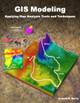
technology and not market-driven solutions following demand. At the moment, the over 500 billion dollar
advertising market with a rapidly growing share in digital media is dominating
attention and the competition for eyeballs is directing geospatial innovation
with a host of new display/visualization capabilities.
User-driven GIS innovation will become more and more
schizophrenic with a growing gap between the two clans of the GIS user
community as shown in figure 1.
Figure
1. Widening gap in the GIS user
community.
Another interesting point is that “radical”
innovation often comes from fields with minimal or no paper map legacy, such as
agriculture and retail sales, because these fields do not have pre-conceived
mapping applications to constrain spatial reasoning and innovation.
In the case of Precision
Agriculture, geospatial technology (GIS/RS/GPS) is coupled with robotics
for “on-the-fly” data collection and prescription application as tractors move
throughout a field. In Geo-business, when you swipe your credit
card an analytic process knows what you bought, where you bought it, where you
live and can combine this information with lifestyle and demographic data
through spatial data mining to derive maps of “propensity to buy” various
products throughout a market area. Keep
in mind that these map analysis applications were non-existent a dozen years
ago but now millions of acres and billions of transactions are part of the
geospatial “stone soup” mix.
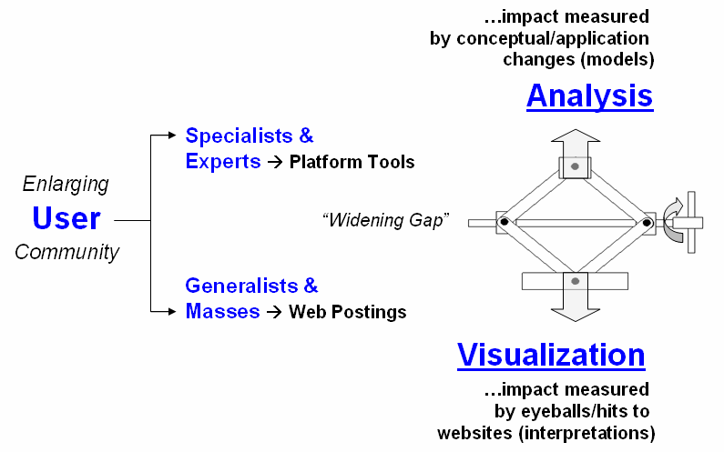
As shown in figure 2 the evolution of GIS is more
cyclical than linear. My greybeard
perspective of over 30 years in GIS suggests that we have been here
before. In the 1970s the research and
early applications centered on Computer
Mapping (display focus) that yielded to Spatial
Data Management (data structure/management focus) in the next decade as we
linked digital maps to attribute databases for geo-query. The 1990s centered on GIS Modeling (analysis focus) that laid the groundwork for whole
new ways of assessing spatial patterns and relations, as well as entirely new
applications such as precision agriculture and geo-business.
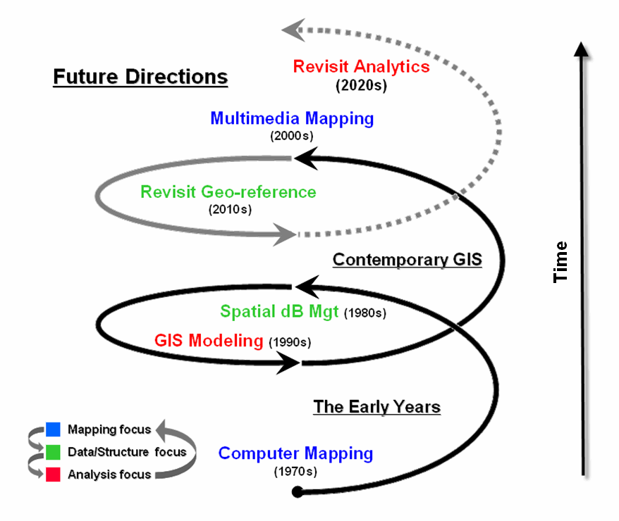
Figure 2. GIS Innovation/Development cycles.
Today, GIS is centered on Multimedia Mapping (mapping focus) which brings us full circle to
our beginnings. While advances in
virtual reality and 3D visualization can “knock-your-socks-off” they represent
incremental progress in visualizing maps that exploit dramatic computer
hardware/software advances. The truly
geospatial innovation waits the next re-focusing on data/structure and analysis.
The bulk of the current state of geospatial analysis
relies on “static coincidence modeling”
using a stack of geo-registered map layers.
But the frontier of GIS research is shifting focus to “dynamic flows modeling” that tracks
movement over space and time in three-dimensional geographic space. But a wholesale revamping of data structure
is needed to make this leap.
The impact of the next decade’s evolution will be
huge and shake the very core of GIS—the Cartesian coordinate system itself …a
spatial referencing concept introduced by mathematician Rene Descartes 400
years ago.
The current 2D square for geographic referencing is
fine for “static coincidence” analysis over relatively small land areas, but
woefully lacking for “dynamic 3D flows.”
It is likely that Descartes’ 2D squares will be replaced by hexagons
(like the patches forming a soccer ball) that better represent our curved
earth’s surface …and the 3D cubes replaced by nesting polyhedrals for a
consistent and seamless representation of three-dimensional geographic
space. This change in referencing
extends the current six-sides of a cube for flow modeling to the twelve-sides
(facets) of a polyhedral—radically changing our algorithms as well as our
historical perspective of mapping (see Author’s Note 1) April
2007 Beyond Mapping column for more discussion).
The new geo-referencing framework provides a needed
foothold for solving complex spatial problems, such as intercepting a nuclear
missile using supersonic evasive maneuvers or tracking the air, surface and
groundwater flows and concentrations of a toxic release. While the advanced map analysis applications
coming our way aren’t the bread and butter of mass applications based on
historical map usage (visualization and geo-query of data layers) they
represent natural extensions of geospatial conceptualization and analysis
…built upon an entirely new set analytic tools, geo-referencing framework and a
more realistic paradigm of geographic space.
____________________________
Author’s Note: 1) For more
discussion, see Beyond Mapping Compilation Series, book IV, Introduction,
Section 3 “Geo-Referencing
Is the Cornerstone of GIS.” 2) I
have been involved in research, teaching, consulting and GIS software
development since 1971 and presented my first graduate course in GIS Modeling
in 1977. The discussion in these columns
is a distillation of this experience and several keynotes, plenary
presentations and other papers—many are posted online at www.innovativegis.com/basis/basis/cv_berry.htm.
GIS and
the Cloud Computing Conundrum
(GeoWorld, September 2009)
I think my first encounter with the concept of cloud
computing was more than a dozen years ago when tackling a Beyond Mapping column
on object-oriented computing. It dealt
with the new buzzwords of “object-oriented” user interface (OOUI), programming
system (OOPS) and database management (OODBM) that promised to revolutionize
computer interactions and code sets (see Author’s Note). Since then there has been a string of new
evolutionary terms from enterprise GIS, to geography network, interoperability,
distributed computing, web-services, mobile GIS, grid computing and mash-ups
that have captured geotechnology’s imagination, as well as attention.
“Cloud computing” is the latest in this trajectory of terminology
and computing advances that appears to be coalescing these seemingly disparate
evolutionary perspectives. While my
technical skills are such that I can’t fully address its architecture or
enabling technologies, I might be able to contribute to a basic grasp of what
cloud technology is, some of its advantages/disadvantages and what its
near-term fate might be.
Uncharacteristic
of the Wikipedia, the definition for cloud computing is riddled with
techy-speak, as are most of the blogs.
However, what I am able to decipher is that there are three
distinguishing characteristics defining it (see figure 1)—
-
it involves virtualized resources
…meaning that workloads are allocated among a multitude of interconnected
computers acting as a single device;
-
it is dynamically scalable …meaning that
the system can be readily enlarged;
-
it acts as a service …meaning that the
software and data components are shared over the Internet.
The result
is a “hosted elsewhere” environment for data and services …meaning that cloud
computing is basically the movement of applications, services, and data from
local storage to a dispersed set of servers and datacenters— an advantageous
environment for many data heavy and computationally demanding applications,
such as geotechnology.
Figure 1. Cloud Computing
characteristics, components and considerations.
A
counterpoint is that the “elsewhere” conjures up visions of the old dumb
terminals of the 70’s connected to an all powerful computer center serving the
masses. It suggests that some of the
tailoring and flexibility of the “personal” part of the PC environment might be
lost to ubiquitous services primarily designed to capture millions of
eyeballs. The middle ground is that
desktop and cloud computing can coexist but that suggests duel markets,
investments, support and maintenance.
Either
way, it is important to note that cloud computing is not a technology—it is a
concept. It essentially presents the
idea of distributed computing that has been around for decades. While there is some credence in the argument
that cloud computing is simply an extension of yesterday’s buzzwords, it
ingrains considerable technical advancement.
For example, the cloud offers a huge potential for capitalizing on the
spatial analysis, modeling and simulation functions of a GIS, as well as
tossing gigabytes around with ease …a real step-forward from the earlier
expressions.
There are two broad types of
clouds depending on their application:
-
“Software as a Service” (SaaS) delivering a single application through the browser to a
multitude of customers (e.g., WeoGeo and Safe Software are making
strides in SaaS for geotechnology)— on the customer side, it means
minimal upfront investment in servers or software licensing and on the provider
side, with just one application to maintain, costs are low compared to
conventional hosting; and,
-
“Utility
Computing” offering
storage and virtual servers that can be accessed on demand by stitching
together memory, I/O, storage, and computational capacity as a virtualized
resource pool available over the Internet— thus creating a development environment for new services and usage
accounting.
Google Earth is a good example of early-stage, cloud-like
computing. It seamlessly stitches
imagery from numerous datacenters to wrap the globe in a highly interactive 3D
display. It provides a wealth of
geography-based tools from direction finding to posting photos and YouTube
videos. More importantly, it has a
developer’s environment (.kml) for controlling the user interface and custom
display of geo-registered map layers. Like
the iPhone, this open access encourages the development of applications and
tools outside the strict confines of dedicated “flagship” software.
But the
cloud’s silver lining has some dark pockets.
There are four very important non-technical aspects to consider in
assessing the future of cloud computing: 1)
liability concerns, 2) information
ownership, sensitivity and privacy issues, 3)
economic and payout considerations, and 4)
legacy impediments.
Liability
concerns
arise from decoupling data and procedures from a single secure computing
infrastructure— what happens if the data is lost or compromised? What if the data and processing are changed
or basically wrong? Who is
responsible? Who cares?
The
closely related issues of ownership, sensitivity and privacy raise
questions like: Who owns the data? Who is it shared with and under what
circumstances? How secure is the
data? Who determines its accuracy,
viability and obsolescence? Who defines
what data is sensitive? What is personal
information? What is privacy? These lofty questions rival Socrates sitting
on the steps of the Acropolis and asking …what is beauty? …what is truth? But these social questions need to be
addressed if the cloud technology promise ever makes it down to earth.
In
addition, a practical reality needs an economic and payout
component. While SaaS is usually
subscription based, the alchemy of spinning gold from “free” cyberspace straw
continues to mystify me. It appears that
the very big boys like Google and Virtual (Bing) Earths can do it through
eyeball counts, but what happens to smaller data, software and service
providers that make their livelihood from what could become ubiquitous? What is their incentive? How would a cloud computing marketplace be
structured? How will its transactions be
recorded and indemnified?
Governments,
non-profits and open source consortiums, on the other hand, see tremendous
opportunities in serving-up gigabytes of data and analysis functionality for
free. Their perspective focuses on
improved access and capabilities, primarily financed through cost savings. But are they able to justify large
transitional investments to retool under our current economic times?
All
these considerations, however, pale in light legacy impediments, such as
the inherent resistance to change and inertia derived from vested systems and
cultures. The old adage “don’t fix it, if it ain’t broke” often
delays, if not trumps, adoption of new technology. Turning the oil tanker of GIS might take a
lot longer than technical considerations suggest—so don’t expect GIS to
“disappear” into the clouds just yet.
But the future possibility is hanging overhead.
_____________________________
Author’s Note: see online book Map Analysis, Topic 1,
Object-Oriented Technology and Its
Visualizing
a Three-dimensional Reality
(GeoWorld, October 2009)
I have always thought of geography in
three-dimensions. Growing up in
California’s high Sierras I was surrounded by peaks and valleys. The pop-up view in a pair of aerial photos
got me hooked as an undergrad in forestry at UC Berkeley during the 1960’s
while dodging tear gas canisters.
My doctoral work involved a three-dimensional computer
model that simulated solar radiation in a vegetation canopy (SRVC). The mathematics would track a burst of light
as it careened through the atmosphere and then bounce around in a wheat field
or forest with probability functions determining what portion was absorbed,
transmitted or reflected based on plant material and leaf angles. Solid geometry and statistics were the
enabling forces, and after thousands of stochastic interactions, the model
would report the spectral signature characteristics a satellite likely would
see. All this was in anticipation of
civilian remote sensing systems like the Earth Resources Technology Satellite
(ERTS, 1973), the precursor to the Landsat program.
This experience further entrenched my view of geography
as three-dimensional. However, the
ensuing decades of GIS technology have focused on the traditional “pancake
perspective” that flatten all of the interesting details into force-fitted
plane geometry.
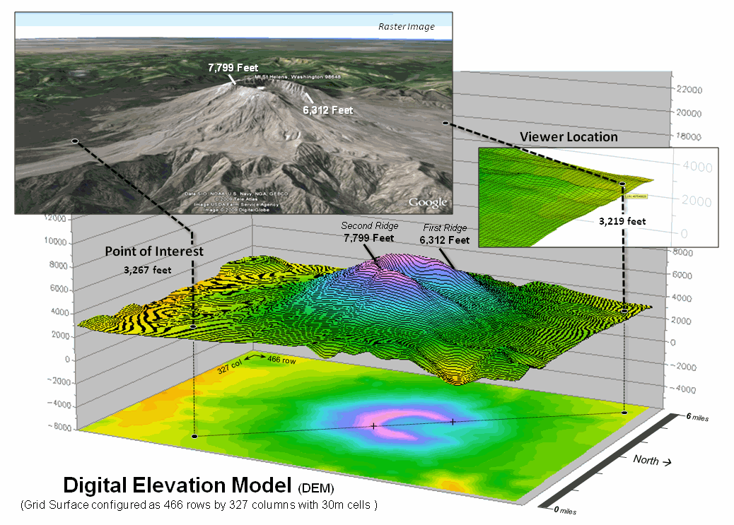
Figure 1. Mount St. Helens topography.
Even more disheartening is the assumption that everything
can be generalized into a finite set of hard boundaries identifying discrete
spatial objects defined by points, lines and polygons. While this approach has served us well for
thousands of years and we have avoided sailing off the edge of the earth,
geotechnology is taking us “where no mapper
has gone before,” at least not without a digital map and a fairly hefty
computer.
Consider
the Google Earth image of Mount St. Helens in the upper-left portion of figure
1. The peaks poke-up and the valleys dip
down with a realistic land cover wrapper.
This three-dimensional rendering of geography is a far cry from the
traditional flat map with pastel colors imparting an abstract impression of the
area. You can zoom-in and out, spin
around and even fly through the landscape or gaze skyward to the stars and
other galaxies.
Underlying
all this is a Digital Elevation Model (DEM) that encapsulates the topographic
undulations. It uses traditional X and Y
coordinates to position a location plus a Z coordinate to establish its
relative height above a reference geode (sea level in this case). However from a purist’s perspective there are
a couple of things that keep it from being a true three-dimensional GIS. First, the raster image is just that— a
display in which thousands the “dumb” dots coalesce to form a picture in your
mind, not an “intelligent” three-dimensional data structure that a computer can
understand. Secondly, the rendering is
still somewhat two-dimensional as the mapped information is simply “draped” on
a wrinkled terrain surface and not stored in a true three-dimensional GIS—a
warped pancake.
The DEM
in the background forms Mt St. Helen’s three-dimensional terrain surface by
storing elevation values in a matrix of 30 meter grid cells of 466 rows by 327
columns (152, 382 values). In this form,
the computer can “see” the terrain and perform its map-ematical magic.
Figure
2 depicts a bit of computational gymnastics involving three-dimensional
geography. Assume you are standing at
the viewer location and looking to the southeast in the direction of the point
of interest. Your elevation is 3,219
feet with the mountain’s western rim towering above you at 6,312 feet and
blocking your view of anything beyond it.
In a sense, the computer “sees” the same thing—except in mathematical
terms. Using similar triangles, it can calculate the minimum point-of-interest height
needed to be visibly connected as (see author’s notes for a link to discussion
of the more robust “splash algorithm” for establishing visual connectivity)…
Tangent = Rise / Run
= (6312 ft – 3219 ft) / (SQRT[(134 – 33)2
+ (454 – 325) 2 ] * 98.4251 ft)
= 3093 ft / (163.835 * 98.4251 ft) = 3893
ft / 16125 ft = 0.1918
Height = (Tangent *
Run) + Viewer Height
= (0.1918 * (SQRT[(300 – 33)2 + (454 – 114) 2
] * 98.4251 ft)) + 3219 ft
= (0.1918 * 432.307 * 98.4251 ft) + 3219
= 11,380 Feet
Since
the computer knows that the elevation on the grid surface at that location is
only 3,267 feet it knows you can’t see the location. But if a plane was flying 11,380 feet over
the point it would be visible and the computer would know it.
Figure 2. Basic geometric relationships determine the
minimum visible height considering intervening ridges.
Conversely,
if you “helicoptered-up” 11,000 feet (to 14,219 feet elevation) you could see
over both of the caldron’s ridges and be visually connected to the surface at
the point of interest (figure 3). Or in
a military context, an enemy combatant at that location would have
line-of-sight detection.
As your
vertical rise increases from the terrain surface, more and more terrain comes
into view (see author’s notes for a link
to an animated slide set). The
visual exposure surface draped on the terrain and projected on the floor of the
plot keeps track of the number of visual connections at every grid surface
location in 1000 foot rise increments.
The result is a traditional two-dimensional map of visual exposure at
each surface location with warmer tones representing considerable visual
exposure during your helicopter’s rise.
However,
the vertical bar in figure 3 depicts the radical change that is taking us
beyond mapping. In this case the
two-dimensional grid “cell” (termed a pixel) is replace by a three-dimensional
grid “cube” (termed a voxel)—an extension from the concept of an area on a
surface to a glob in a volume. The
warmer colors in the column identify volumetric locations with considerable
visual exposure.
Figure 3. 3-D
Grid Data Structure is a
direct expansion of the 2D structure with X, Y and Z coordinates defining the
position in a 3-dimensional data matrix plus a value representing the
characteristic or condition (attribute) associated with that location.
Now
imagine a continuous set of columns rising above and below the terrain that
forms a three-dimensional project extent—a block instead of an area. How is the block defined and stored; what new
analytical tools are available in a volumetric GIS; what new information is
generated; how might you use it? …that’s fodder for the next section. For me, it’s a blast from the past that is
defining the future of geotechnology.
____________________________
Author’s Notes: for a more detailed discussion of visual
connectivity see the online book Beyond Mapping III, Topic 15, “Deriving and Using
Visual Exposure Maps” at www.innovativegis.com/basis/MapAnalysis/Topic15/Topic15.htm. An
annotated slide set demonstrating visual connectivity from increasing viewer
heights is posted at www.innovativegis.com/basis/MapAnalysis/Topic27/AnimatedVE.ppt.
Thinking
Outside the Box
(GeoWorld, November 2009)
Last section used a progressive series of line-of-sight
connectivity examples to demonstrate thinking beyond a 2-D map world to a
three-dimensional world. Since the
introduction of the digital map, mapping geographic space has moved well beyond
its traditional planimetric pancake perspective that flattens a curved earth
onto a sheet of paper.
A
contemporary Google Earth display provides an interactive 3-D image of the
globe that you can fly through, zoom-up and down, tilt and turn much like Luke
Skywalker’s bombing run on the Death Star.
However both the traditional 2-D map and virtual reality’s 3-D
visualization view the earth as a surface—flattened to a pancake or curved and
wrinkled a bit to reflect the topography.
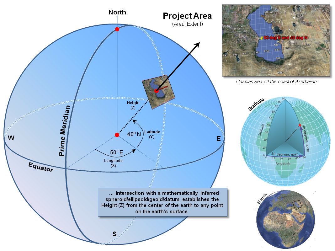
Figure 1. A 3-dimensional
coordinate system uses angular measurements (X,Y) and length (Z) to locate
points on the earth’s surface.
Figure
1 summarizes the key elements in locating yourself on the earth’s surface …sort
of a pop-quiz from those foggy days of Geography 101. The Prime Meridian and Equator serve as base references
for establishing the angular movements expressed in degrees of Longitude (X)
and Latitude (Y) of an imaginary vector from the center of the earth passing
through any location. The Height (Z) of
the vector positions the point on the earth’s surface.
It’s
the determination of height that causes most of us to trip over our geodesic
mental block. First, the globe is not a
perfect sphere but is a squished ellipsoid that is scrunched at the poles and
pushed out along the equator like love-handles.
Another way to conceptualize the physical shape of the surface is to
imagine blowing up a giant balloon such that it “best fits” the actual shape of
the earth (termed the geoid) most often aligning with mean sea level. The result is a smooth geometric equation
characterizing the general shape of the earth’s surface.
But the earth’s mountains bump-up and valleys bump-down
from the ellipsoid so a datum is designed to fit the earth's
surface that accounts for the actual wrinkling of the globe as recorded by
orbiting satellites. The most common datum for the world is WGS 84 (World
Geodetic System 1984) used by all GPS
equipment and tends to have and accuracy of +/- 30 meters or less from the
actual local elevation anywhere on the surface.
The
final step in traditional mapping is to flatten the curved and wrinkled surface
to a planimetric projection and plot it on a piece of paper or display on a
computer’s screen. It is at this stage
all but the most fervent would-be geographers drop the course, or at least drop
their attention span.
However,
a true 3-D GIS simply places the surface in volumetric grid elements along with
others above and below the surface. The
right side of figure 2 shows a Project Block containing a million grid elements
(termed “voxels”) positioned by their geographic coordinates—X (easting), Y
(northing) and Z (height). The left side
depicts stripping off one row of the elevation values defining the terrain
surface and illustrating a small portion of them in the matrix by shading the
top’s of the grids containing the surface.
At
first the representation in a true 3-D data structure seems trivial and
inefficient (silly?) but its implications are huge. While topographic relief is stable (unless
there is another Mount St. Helens blow that redefines local elevation) there
are numerous map variables that can move about in the project block. For example, consider the weather “map” on
the evening news that starts out in space and then dives down under the rain
clouds. Or the National Geographic show
that shows the Roman Coliseum from
above then crashes through the walls to view the staircases and then proceeds
through the arena’s floor to the gladiators’ hypogeum with its subterranean network of tunnels and cages.
Some “real cartographers” might argue that those aren’t
maps but just flashy graphics and architectural drawings …that there has been a
train wreck among mapping, computer-aided drawing, animation and computer
games. On the other hand, there are
those who advocate that these disciplines are converging on a single view of
space—both imaginary and geographic. If
the X, Y and Z coordinates represent geographic space, nothing says that Super
Mario couldn’t hop around your neighborhood or that a car is stolen from your
garage in Grand Theft Auto and race around the streets in your hometown.
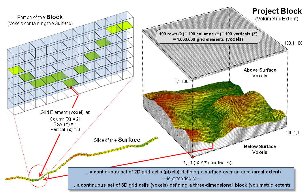
Figure 2. An implied 3-D matrix
defines a volumetric Project Block, a concept analogous to areal extent in
traditional mapping.
The
unifying concept is a “Project Block” composed of millions of
spatially-referenced voxels.
Line-of-sight connectivity determines what is seen as you peek around a
corner or hover-up in a helicopter over a mountain. While the mathematics aren’t for the
faint-hearted or tinker-toy computers of the past, the concept of a “volumetric
map” as an extension of the traditional planimetric map is easy to grasp—a bunch
of three-dimensional cubic grid elements extending up and down from our current
raster set of squares (bottom of figure 3).
However,
akin to the seemingly byzantine details in planimetric mapping, things aren’t
that simple. Like the big bang of the
universe, geographic space expands from the center of the earth and a simple
stacking of fixed cubes like wooden blocks won’t align without significant
gaps. In addition, the geometry of a
cube does not have a consistent distance to all of its surrounding grid
elements and of its twenty six neighbors only six share a complete side with
the remaining neighbors sharing just a line or a single point. This inconsistent geometry makes a cube a
poor grid element for 3-D data storage.
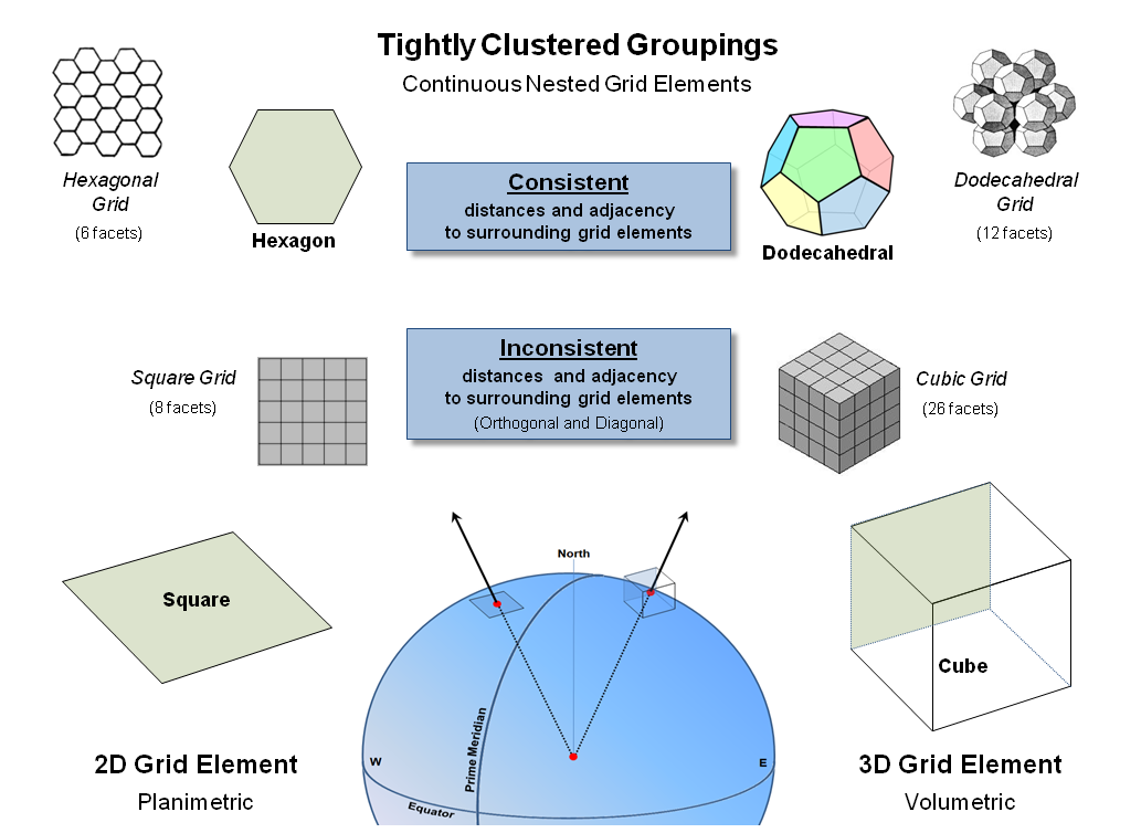
Figure 3. The hexagon and dodecahedral are alternative
grid elements with consistent nesting geometry.
Similarly,
it suggests that the traditional “square” of the Cartesian grid is a bit
limited—only four complete sides (orthogonal elements) and four point
adjacencies (diagonal). Also, the
distances to surrounding elements are different (a ratio of 1:1.414). However, a 2D hexagon shape (beehive honey
comb) abuts completely without gaps in planimetric space (termed “fully
nested”); as does a combination of pentagon and hexagon shapes nests to form
the surface of a spheroid (soccer ball).
To help
envision an alternative 3-D grid element shape (top-right of figure 3) it is helpful
to recall Buckminster Fuller's book Synergetics and his classic treatise of various "close-packing"
arrangements for a group of spheres.
Except in this instance, the sphere-shaped grid elements are replaced by
"pentagonal dodecahedrons"— a set of uniform solid shapes with 12
pentagonal faces (termed geometric “facets”) that when packed abut completely
without gaps (termed fully “nested”).
All of
the facets are identical, as are the distances between the centroids of the
adjoining clustered elements defining a very “natural” building block (see
Author’s Note). But as always, “the
Devil is in the details” and that discussion is reserved for another time.
_____________________________
Author’s Note: In 2003, a team of cosmologists and
mathematicians used NASA’s WMAP cosmic background radiation data to develop a
model for the shape of the universe. The
study analyzed a variety of different shapes for the universe, including finite
versus infinite, flat, negatively- curved (saddle-shaped), positively- curved
(spherical) space and a torus (cylindrical). The study revealed that the
math adds up if the universe is finite and shaped like a pentagonal
dodecahedron (http://physicsworld.com/cws/article/news/18368). And
if one connects all the points in one of the pentagon facets, a
5-pointed star is formed. The ratios of the lengths of the resulting line
segments of the star are all based on phi, Φ, or 1.618… which is the
“Golden Number” mentioned in the Da Vinci Code as the universal constant of
design and appears in the proportions of many things in nature from DNA to the
human body and the solar system—isn’t mathematics wonderful!
_____________________
Further Online Reading: (Chronological listing posted at www.innovativegis.com/basis/BeyondMappingSeries/)
From a Map Pancake to a Soufflé — continues
the discussion of concepts and configuration of a 3D GIS (December 2009)
(Back
to the Table of Contents)