|
Introduction –
Extending Basic GIS Concepts |
GIS
Modeling book |
Finding
Common Ground in Paper and Digital Worlds — describes
the similarities and differences in information and organization between
traditional paper and digital maps
Understand
Resolution to “Think with Maps” — discusses the factors that
determine the “informational scale” digital maps
Geo-Referencing
Is the Cornerstone of GIS — describes current and
alternative approaches for referencing geographic and abstract space
Further Reading
— two additional sections
<Click here>
for a printer-friendly version of this
topic (.pdf).
(Back to the Table of Contents)
______________________________
Finding Common Ground in Paper and Digital Worlds
(GeoWorld, February 2007)
In the
real world, landscapes are composed rocks, dirt, water, green stuff and
furry/feathered friends. In a “paper
world” these things are represented by words, tables and graphics. The traditional paper map is a graphical representation
with inked lines, shadings and symbols used to locate landscape features using
three basic building blocks— Points, Lines and Areas. For example, a
typical water map might identify a well as a dot, a stream as a squiggle and a
lake as a blue blob (figure 1). Each
feature is considered a well-defined “discrete spatial object” with unique
spatial character, positioning and dimension.
In
geometry a point is considered dimensionless, however, the corresponding
concept in cartography is a dot of ink having a physical dimension of a few
inches to several miles depending on the scale of a paper map. Similarly, a line in mathematical theory has
only length but is manually mapped as a thin serpentine polygon of the pen’s
width. An area feature has both length
and width in two-dimensional space. The
interplay of mapping precision and accuracy in a digital world involves a
discussion of scale and resolution reserved for the next section. For now, let’s consider the revolutionary
changes in map form and content brought on by the digital map as outlined in
the rest of figure 1.
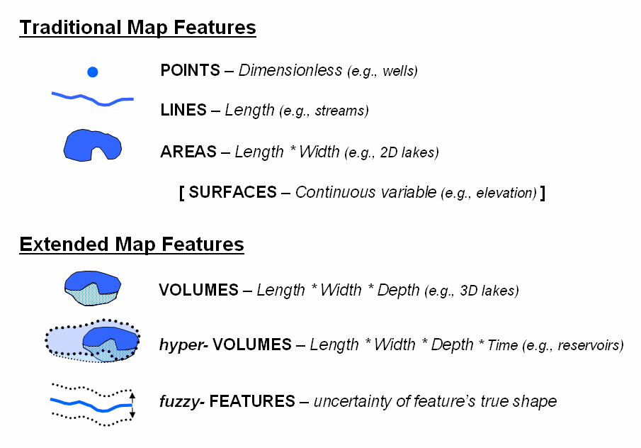
Figure 1. Traditional and Extended Map Features.
For
thousands of years, manual cartography has been limited to characterizing all
geographic phenomena as discrete 2-dimensional spatial objects. However many map variables, such as
elevation, change continuously and representation as contour lines suggests a
nested series of flat layers like a wedding cake instead of the actual
continuously undulating terrain. The
introduction of a grid-based data structure provides for a new basic building
block—a map Surface of continuously
changing values throughout geographic space.
Another
extension to the building blocks is Volumes
that track length, width and depth in characterizing discrete or continuous
variables in 3-dimensional space. For
example, the Length (x-axis), Width (y-axis), Depth (z-axis) coordinates
identify a specific location in a lake and a fourth value (attribute) can
identify its temperature, turbidity, salinity or other condition.
A hyper-Volume (or hyper-point, -line,
-area or -surface) introduces time as an additional abstract coordinate. For example, the weekly water volume of a
reservoir might be tracked by L,W,D,T coordinates identifying a location in
3-dimensional space, as well as time combined with a fifth attribute value
indicating whether water is present or not.
This conceptual extension is a bit tricky and provides conceptual fodder
about mixed referencing units (e.g., meters and minutes) for a subsequent
discussion. However, the result is a
discrete volumetric map feature that shrinks and expands throughout a year—a
dynamic spatial entity that at first appears to violate orthodox mapping
commandments.
Another
mind-bend brought on by the digital map is the concept of fuzzy-features. This idea
tracks the certainty of a feature or condition at each map location. For example, the boundary line of a soil
polygon is a subjective interpretation, while soil parcel’s actual edge could
be a considerable distance away—“the boundary is likely here (high probability)
but could be over there (low probability).”
Another fuzzy example is a classified satellite image where statistical
probabilities are used to establish which cover type is most likely.
Taken
to the hilt, one can conceptualize a data structure that carries L,W,D,T and
A,P (attribute and probability) descriptors that identify a location in space
and time, as well as characterize its most likely condition, next most likely,
and so on—sort of a sandwich of probable conditions. Such a representation challenges the
infallible paradigm of mapping but opens a whole new world of error propagation
modeling.
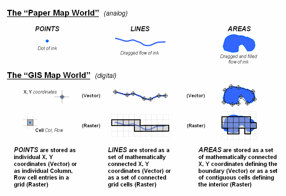
Figure 2. Basic Vector and Raster Data Structure
Considerations.
Whereas
volumes, hyper-volumes and fuzzy-features define the current realm of GIS
researchers, an understanding of contemporary approaches for characterizing
points, lines, and areas is necessary for all GIS users. Figure 2 outlines the two fundamental
approaches—vector and raster (see Author’s Notes).
A Point defined by X,Y coordinates in
vector, and a Cell defined by Col,Row
indices in raster, form the basic data structure units—the “smallest
addressable unit of space” in a map.
Lines are formed by mathematically connecting points (vector) or
identifying all of the conjoined cells containing a line (raster). Areas are defined by a set of points that
define a closed line encompassing a feature (vector) or by all of the
contiguous cells containing a feature (raster).
While
spatial precision is a major operational difference between vector and raster
systems, how they characterize geographic space is important in understanding
limitations and capabilities. Vector
precisely identifies critical points along a line, but the intervening
connections are implied. Raster, on the
other hand, identifies all of the cells containing a line without any implied gaps. Similarly, vector precisely stores an area’s
boundary but implies its interior (must calculate); raster stores the interior
but implies the boundary (must calculate).
The
differences in “what is defined” and “what is implied” determine just about everything
in GIS technology, except maybe the color pallet for display—data structure,
storage requirements, algorithms, coding and ultimately appropriate use. Vector systems precisely and efficiently
store traditional discrete map objects, such as underground cables and property
boundaries (mapping and inventory).
Raster systems, on the other hand, predefine continuous geographic space
for rapid and enhanced processing of map layers (analysis and modeling).
So how
do you think vector and raster systems store surfaces, volumes, hyper-volumes
and fuzzy-features? …very poorly, or not at all for vector systems. However raster systems pre-define all of a
project area (no gaps) by carrying a thematic value for each cell in a
2-dimensional storage matrix to form a continuous
map surface. For volumes, a third
geographic referencing index is added to extend the 2D cells to 3D cubes in
geographic space defined by their X,Y,Z position in the storage matrix see
Author’s Notes).
A
similar expansion is used for hyper-volumes with four indices (X,Y,Z,T)
identifying the “position,” except in this instance an abstract space is
implied due to the differences in geographic and time units. Information about fuzzy-features can be coded
into a compound attribute value describing any map feature, where the first few
digits identify the character/condition at a location with the trailing two
digits identifying the certainty of classification.
The
bottom line is that tomorrow’s maps aren’t simply colorful electronic versions
of your grandfather’s maps. The digital
map is an entirely different beast supporting radically new mapping approaches,
perspectives, opportunities and responsibilities.
_____________________________
Author’s Notes: Topic 6,
“Alternative Data Structures,” in Beyond Mapping Series book II (hardcopy book,
Spatial Reasoning for Effective GIS (Berry 1995, Wiley)) contrasts
vector and raster data structures and describes related alternative structures
including TIN, Quadtree, Rasterized Lines and Vectorized Cells.
Understand
Resolution to “Think with Maps”
(GeoWorld, March 2007)
One of
the most fundamental concepts in the paper map world is Geographic Scale—the relationship between a distance on a map and
its corresponding distance on the earth.
In equation form, scaleratio=
map distance / ground distance but is often expressed as a representative
fraction (RF), such as scaleRF=
1:63,360 meaning 1 inch on the map represents 63,360 inches (or 1 mile) on
the earth’s surface.
However
in the digital map world, this traditional concept of scale does not
exist. While at first this might seem
like cartographic heresy, note that the “map distance” component of the
relationship is assumed to be fixed as ink marks on paper. In a GIS, however, the map features are
stored as organized sets of numbers representing their spatial position
(coordinates for “where”) and thematic attribute (map values for “what”). One can zoom in and out on the data thereby
creating a continuous gradient of geographic scales in the resulting display or
hardcopy plot.
Hence
geographic scale is a function of the display, not an inherent property of the
digital mapped data set. What is important
is the implied concept of informational scale, or Resolution—the ability to discern detail. Traditionally it is implicit that as
geographic scale decreases, resolution also diminishes since drafted feature
boundaries must be smoothed, simplified or not shown at all due to the width of
the inked lines.
However
in a GIS, the concept of resolution is explicit. In fact there are five types of resolution
that need to be considered—Spatial, Mapping, Thematic, Temporal and Model. Spatial
Resolution is the most basic and identifies the “smallest addressable unit”
of geographic space (figure 1). For
point features, the X,Y coordinates (vector) and cell size (raster) determine
the smallest addressable unit.
For
line features in vector, however, the smallest addressable unit is the line
segment with larger segments capturing less detail as the implied straight line
misses the subtle wiggles and waggles of a pattern. Similarly, large grid cells capture less
linear detail than smaller cells.
Figure 1. Spatial Resolution
describes the level of positional detail used to track a geographic pattern or
distribution.
Figure 2. Minimum Mapping
Resolution describes the level of physical aggregation used to depict a
geographic pattern or distribution.
For
polygon features in vector, an entire polygon represents the smallest
addressable unit as the boundary needs to be completed before the implied
interior condition can be identified. In
raster, the smallest addressable unit is defined by the cell size as the
condition is carried for each of the cells comprising the interior and edge of
a polygon feature.
The
concept of spatial resolution easily extends to the level of spatial
aggregation or Minimum Mapping Resolution
that identifies the “smallest physical grouping” of a map theme (figure
2). For example, a high resolution
forest map might identify individual trees (very small polygons delineating
canopy extent), whereas more generally, numerous trees are used to identify a
forest parcel of several acres that ignores the scattered tree
occurrences. The size of the minimum
polygon is determined by the interpretation process with smaller groupings
capturing more detail of the pattern and distribution.
Thematic Resolution identifies
the “smallest classification grouping” of a map theme. For example, a simple forest/non-forest map
might provide a sufficient description of vegetation for some uses and this
coarse classification has appeared for years as green on USGS topographic
sheets. However, resource managers
require a higher thematic resolution of vegetation cover and expand the
classification scheme to include species, age, stocking level and other
characteristics. The result is a finer
set of classification categories of a generalized forest area into smaller more
detailed parcels (figure 3).
Figure 3. Thematic Resolution
describes the level of classification aggregation used to depict a geographic
pattern or distribution.
A
fourth consideration involves Temporal
Resolution that identifies the frequency, or time-step of map update. Some data types, such as geological and
landform maps, change very slowly and do not need frequent revision. A city planner, on the other hand, needs land
use maps that are updated every couple of years and include future development
sites. A retail marketer needs even higher
temporal resolution and will likely update sales and projection figures on a
monthly, weekly or even daily basis.
Model Resolution is the
least defined and involves factors affecting the level of detail used in
creating a derived map, such as an optimal corridor for an electric
transmission line or areas of suitable wildlife habitat. Model resolution considers detail ingrained
in 1) the interpretation/analysis assumptions (logic) and 2) the
algorithms/procedures (processing) used in implementing a spatial model. For example, a proposed transmission line
could be routed considering just terrain steepness for a low model resolution,
or extended to include other engineering factors (soils, road proximity, etc.),
environmental concerns (wetlands, wildlife habitats, etc.) and social
considerations (visual exposure, housing density, etc.) for much higher model
resolution.
So why
should we care about digital map resolution?
Because accounting for informational scale is just as important as
adjusting for a common geographic scale and projection when interacting with a
stack of maps. Our paper map heritage
focused on descriptive mapping (inventory of physical phenomena) whereas an
increasing part of the GIS revolution focuses on prescriptive mapping (spatial
relationships of physical and cognitive interactions). This “thinking with maps” requires a thorough
understanding of the spatial, map, thematic, temporal and model resolutions of
the maps involved or you will surely be burned.
Geo-Referencing
Is the Cornerstone of GIS
(GeoWorld, April 2007)
In the
mid-1600s the French mathematician, René
Descartes established the Cartesian coordinate system that is still in use
today. The system determines the location of each point in a plane as defined
by two numbers—a “x-coordinate”
and a “y-coordinate.”
A third z-coordinate
is used to extend the system to 3-dimensional geographic space (see Author’s
Notes). In mapping, these coordinates reference
a
refined ellipsoid (geodetic datum) that can be
conceptualized as a curved surface approximating the mean ocean surface of the
earth.
The location and shape of map features can be established
by X and Y distances measured along flattened portions of the reference surface
(figure 1). The familiar Universal
Transverse Mercator (UTM) coordinates
represent E-W and N-S movements in meters along the plane. The rub is that UTM zones are need to break
the curved earth surface into a series of small flat, projected subsections
that are difficult to edge-match.
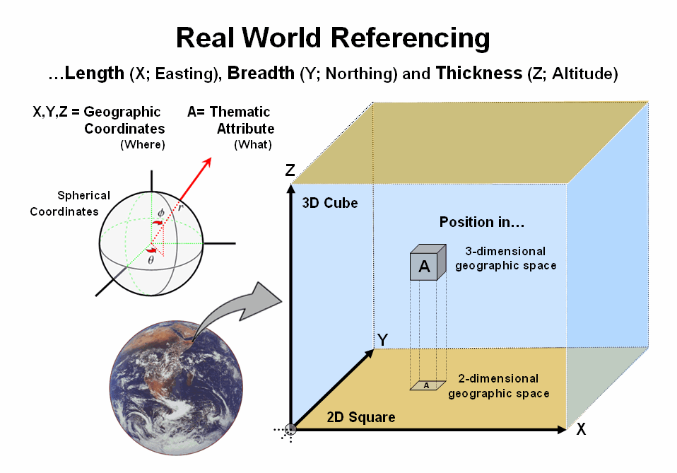
Figure 1. Geographic referencing
uses three coordinates to locate map features in real world space.
A
variant of the traditional referencing system uses spherical coordinates that
are based on solid angles measured from the center of the earth. This natural form for describing positions on
a sphere is defined by three coordinates—an azimuthal
angle (θ) in the X,Y plane from the x-axis, the polar angle
(φ) from the z-axis, and the radial
distance (r) from the earth’s center (origin). The advantage of a spherical referencing
system is that it is seamless throughout the globe and doesn’t require
projecting to a localized flat plane.
Digital map storage is rapidly
moving toward spherical referencing that uses latitude and longitude in decimal
degrees for internal storage and on-the-fly conversion to any planar
projection. This radical change from our
paper map heritage is fueled by ubiquitous
use of GPS and a desire for global databases that easily walk across political
and administrative boundaries.
Since the digital map is a radical departure from the
paper map, other alternative referencing schemes are possible. For example, hexagons can replace the
Cartesian grid squares we have used for hundreds of years (top portion of
figure 2). The hexagon naturally nests
to form a continuous network like a beehive’s honeycomb. An important property of a hexagon grid is
that it better represents curved surfaces than a square grid— a soccer ball
stitched from squares wouldn’t roll the same [Note: actually a soccer ball is a composite of hexagons (white) and
pentagons (black)].
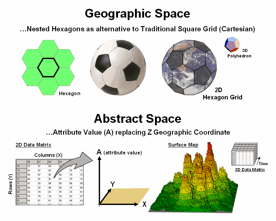
Figure 2. Alternative referencing systems and abstract
space characterization are possible through the digital nature of modern maps.
However the most important property is that a hexagon has
six sides instead of four. The added
directions provide a foothold for more precise measurement of continuous
movement— one can turn right- and left-oblique as well as just right and
left. Traditional routing models using
Least Cost Path would benefit greatly.
Expanding to 3-dimensional geographic space provides for
polyhedrons to replace cubes. For
example, a dodecahedron
is a nesting twelve-sided object that can be used instead of the six-sided
cube. Weather and ground water flow
modeling could be greatly enhanced by the increased options for transfer from a
location to its larger set of adjoining locations. The computations for cross-products of
vectors, such as warp-speed cruise missiles, could be greatly assisted as they
are affected by different atmospheric conditions and evasive trajectories.
Another
extension involves the use of abstract space (bottom portion of figure 2). For example, the Z-coordinate can be replaced
with an attribute value to generate a map surface, such as customer
density. In this instance, the abstract
referencing is a mixture of spatial and attribute “coordinates” and doesn’t
imply 3-dimensional, real word geographic occurrences. Instead, it relates geography and conditions
in an extremely useful way for conceptualizing patterns. Normalization along the abstract coordinate
axis is an important consideration for both visualization and analysis.
This
brings us to space-time referencing.
During a recent panel discussion I was challenged for suggesting such a
combination is possible within a GIS.
The idea has been debated for years by philosophers and physicists but
H.G. Wells’ succinct description is one of the best—
'Clearly,' the Time Traveller proceeded,
'any real body must have extension in four directions: it must have Length,
Breadth, Thickness, and - Duration. But through a natural infirmity of the
flesh, which I will explain to you in a moment, we incline to overlook this
fact. There are really four dimensions, three which we call the three planes of
Space, and a fourth, Time. There is, however, a tendency to draw an unreal
distinction between the former three dimensions and the latter, because it
happens that our consciousness moves intermittently in one direction along the
latter from the beginning to the end of our lives.' (Chapter 1, Time Machine).
The
upshot seems to be that a fourth dimension exists (see Author’s Notes), it is
just you can’t go there in person. But a
GIS can easily take you there—conceptually that is. For example, an additional abstract “coordinate”
representing time can be added to form a 3-dimensional data matrix. The GIS picks off the customer density data
for the first “page” and displays it as in the figure. Then it uses the data on the on the second
page (one time step forward) and displays it.
This is repeated to cycle through time and you see an animation where
the peaks and valleys of the density surface move with time.
So
animation enables you to move around a city (X,Y) viewing the space-time
relationship of customer density (A). In
a similar manner you could evaluate a forest “green-up” model to predict re-growth
at a series of time steps after harvesting to look into future landscape
conditions. Or you can watch the
progression over time of ground water pollutant flow in 3D space (4D data
matrix) using a semi-transparent dodecahedron solid grid just for fun and
increased modeling accuracy. In fact, it
can be argued that GIS is inherently n-dimensional
when you consider a map stack of multiple attributes and time is simply another
abstract dimension.
My
suspicions are that revolutions in referencing will be a big part of GIS’s
frontier in the 2010s. See you there?
_____________________________
Author’s Notes: an excellent online reference for the basic
geometry concepts underlying traditional and future geo-referencing techniques
is the Wolfram MathWorld pages, such as the posting describing the dodecahedron
at http://mathworld.wolfram.com/Dodecahedron.html;
a
_____________________
Further Online Reading: (Chronological listing posted at www.innovativegis.com/basis/BeyondMappingSeries/)
Is it Soup Yet? — describes
the evolution in GIS definitions and terminology (February 2009)
What’s in a Name — suggests
and defines the new more comprehensive term “Geotechnology” (March 2009)
(Back
to the Table of Contents)