|
Beyond
Mapping IV Topic 8
– GIS Modeling in Natural Resources (Further Reading) |
GIS Modeling book |
A Twelve-step Program for
Recovery from Flaky Forest Formulations — describes
a spatial model for identifying Landings and Timbersheds (June 2010)
Bringing
Travel and Terrain Directions into Line —
describes comparison procedures and route evaluation techniques (December 2012)
Optimal
Path Density is not all that Dense (Conceptually) — uses Optimal Path
Density Analysis to identify “corridors of common access” (January 2013)
Assessing
Wildfire Response (Part 1): Oneth
by Land, Twoeth by Air — discusses
a spatial model for determining effective helicopter landing zones (August 2011)
Assessing
Wildfire Response (Part 2): Jumping Right into It — describes map analysis procedures
for determining initial response time for alternative attack modes (September 2011)
<Click here> for a printer-friendly version of this topic (.pdf).
(Back
to the Table of Contents)
______________________________
A Twelve-step Program for
Recovery from Flaky Forest Formulations
(GeoWorld, June
2010)
Earlier discussions (“Harvesting an Understanding of GIS Modeling,”
GeoWorld April 2010 and “Extending Forest Harvesting’s Reach,” GeoWorld
May 2010) described a basic spatial model for determining forest availability
and access considering physical and legal factors that, in turn, was extended
to include human concerns of housing density and visual exposure to harvesting
activity. This section builds on those
procedures for a further formulated model that 1) identifies the best set of
staging areas for wood collection, termed “Landings” and 2) delineates
the harvest areas optimally connected to each landing, termed “Timbersheds.”
The model involves logical sequencing of twelve standard map analysis
steps that are described using MapCalc commands that are easily translated into
other grid-based software systems (see author’s note). The top portion of figure 1 uses the five
“binary maps” created in the basic model to generate a map of potential landing
areas. The maps are calibrated as 1 =
available and 0 = not available for harvesting, and when multiplied together (1.
Compute) results in 1 being assigned to all roads locations passing through
available forest areas— 1*1*1*1*1= 1; if a zero appears in any map layers it
results in a 0 value (not a road in an available forest area).
Figure 1. Identifying candidate Landing Sites that are
along forested roads in gently sloped areas (steps 1-3).
The lower portion of figure 1 depicts using a neighborhood/focal
summary operation (2. Scan) to calculate the average slope within a
100-foot reach of the each forested road cell.
The third step (3. Renumber) eliminates potential landing areas
that that are in areas with fairly steep surrounding terrain (> 15% average
slope). The result is removal of over
two thirds of the total number of road locations.
Figure 2 shows processing steps 4 through 9 used to locate the best
landing sites. In step 4, the Discrete
Cost map indicating the relative ease of equipment operation created in the
basic model is masked (4. Compute) to constrain harvesting activity to
just the forested areas. The
Accumulated Proximity from roads is calculated (5. Spread) resulting in
an effective distance value for each forest location that respects the
intervening terrain conditions from forested roads.
The optimal path from each forest location to its nearest road location
is determined and the set of paths are counted for each map location (6.
Drain) resulting in an Optimal Path Density surface. The insets in the upper-right portion of
figure 2 shows 2D and 3D displays of this less-than-intuitive surface. Note the yellow and red tones where many
forest locations are optimally accessed—with one road location in the southern
portion of the project area servicing 785 forested locations. The long red path leading to this location is
analogous to a primary road where more and more collector streets join the
overall best route.
The summary statistics, along with expert judgment is used to identify
an appropriate final set of landing sites that is suitably dispersed throughout
the project area (10. Renumber) as depicted in the upper portion of
figure 3. These final locations for Landings
are used to derive new effective distance values for each forest location
considering intervening terrain conditions (11. Spread) in a manner
similar to step 5. Finally, expert
judgment is used to limit the reach in each of the Timbersheds to a manageable
distance (12. Renumber).
Figure 2. Locating the best
Landing Sites based on optimal path density (steps 4-9).
The lower portion of figure 2 shows the steps for isolating the best
landing sites. The highest levels of
optimal path density are isolated (7. Renumber) and then masked to
identify the forested road locations with the highest optimal path density (8.
Compute). In turn these locations
are assigned a unique ID value (9. Clump) and summary statistics on each
of the “best” potential landing sites are generated.
To put the spatial analysis into a decision context, a “thumbnail”
estimate of the wood chip resource for Timbershed #15 is 164ac * 40T/ac = 6560
tons. At $15 to $30 per ton this converts
to 6560T * $22.50 = $147,600. From
another perspective, assuming 6000 to 8000 btu per pound of woodchips the
energy stored in the biomass translates to 6560T * 2000lb/T * 7000btu/lb =
91,840,000,000 btu. At 3412 btu per
kilowatt hour this converts to 91,840,000,000btu / 3412btu/kWh = nearly 27
million kilowatt hours …whew!
Any way you look at it there is a lot of energy locked up in the
giga-tons of beetle-gnawed biomass blanketing the Rockies. GIS modeling of its availability and access
is but one of several critical steps needed in determining the economic,
environmental and social viability of a “wood utilization” solution.
Figure 3. Identifying and
characterizing the Timbersheds of the best Landing Sites (steps 10-12).
_____________________________
Author’s
Note: See http://www.innovativegis.com/basis/MapCalc/MCcross_ref.htm
for cross-reference of MapCalc commands to other software systems. An animated
PowerPoint slide set of this 3-part Beyond Mapping series on “Assessing and Characterizing
Relative Forest Access” and materials for a “hands-on” exercise are posted at www.innovativegis.com/basis/MapAnalysis/Topic29/ForestAccess.htm.
Bringing Travel and Terrain Directions into Line
(GeoWorld,
December 2012)
Precious discussions addressed “Backcountry 911” that considers both
on- and off-road travel for emergency response (“E911 for the
Backcountry,” GeoWorld, July 2010; “Extending Emergency Response
Beyond the Lines,” GeoWorld, August 2010; “Comparing Emergency Response
Alternatives,” GeoWorld September 2010). As
identified in the left portion of figure 1, the analysis involves the
development of a “stepped accumulation surface” that first considers on-road
travel by assigning the minimum travel-time from headquarters to all of the
road locations. As shown in the figure,
the farthest away location considering truck travel is 26.5 minutes occurring
in the southeast corner of the project area.
The next step considers disembarking anywhere along the road network
and moving off-road by ATV. However, the
ability to simulate different modes of travel is not available in most
grid-based map analysis toolsets. The
algorithm requires the off-road movement to “remember” the travel-time at each
road location and then start accumulating additional travel-time as the new
movement twists, turns, and stops with respect to the relative and absolute
barriers calibrated for ATV off-road travel (see Author’s Note 2).
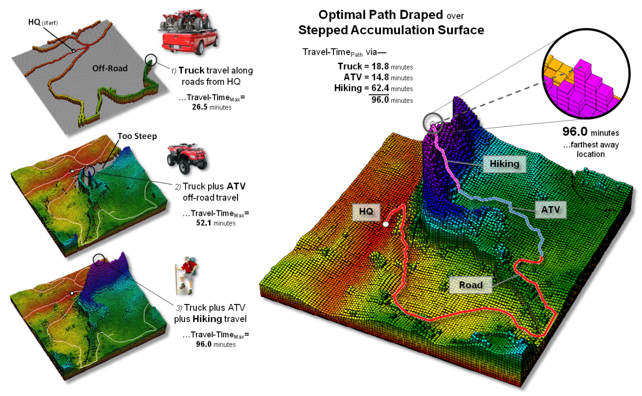
Figure 1. A backcountry emergency
response surface identifies the travel-time of the “best path” to all locations
considering a combination of truck, ATV and hiking travel.
The middle-left inset in figure 1 shows the accumulated travel-time for
both on-road truck and off-road ATV travel where the intervening terrain
conditions act like “speed limits” (relative barriers). Also, ATV travel is completely restricted by
open water and very steep slopes (absolute barriers). The result of the processing assigns the
minimum total travel-time to all accessible locations comprising about 85% of
the project area. The farthest away
location assuming combined truck and ATV travel is 52.1 minutes occurring in
the central portion of the project area.
The remaining 15% is too steep for ATV travel and necessitates hiking
into these locations. In a similar
manner, the algorithm picks up the accumulated truck/ATV travel-time values and
moves into the steep areas respecting the hiking difficulty under the adverse
terrain conditions. Note the large
increases in travel-time in these hard to reach areas. The farthest away location assuming combined
truck, ATV and hiking is 96.0 minutes, also occurring in the central portion of
the project area.
A traditional accumulation surface (one single step) identifies the
minimum travel-time from a starting location to all other locations considering
“constant” definitions of the relative and absolute barriers affecting
movement. It has two very unique
characteristics— 1) it forms a bowl-like shape with the starting point (or points)
having the lowest value of zero = 0 units away from the start, and 2)
continuously increasing travel-time values reflecting the relative ease of
movement that warps the bowl with areas of relatively rapid increases in
travel-time associated with areas of high relative barrier “costs.”
A stepped accumulation surface (top-center portion of figure 2) shares
these characteristics but is far more complex as it reflects the cumulative
effects of different modes of travel and the impact of their changing relative
and absolute barriers on movement. Note
the dramatic “ridge” running NE-SW through the center of the project area, as
well as the other morphological ups and downs in total combined travel-time.
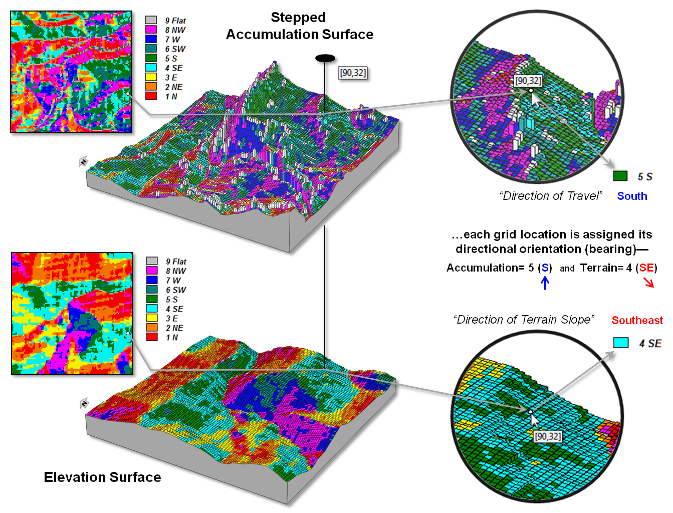
Figure 2. Maps of travel and
terrain direction are characterized by the aspect (bearings) of their
respective surfaces.
In a sense, this wrinkling is analogous to a terrain surface, but the
surface’s configuration is the result of the relative ease of on- and off-road
travel in cognitive space— not erosion, fracture, slippage and subsidence of
dirt in real world space.
However like a terrain surface, an “aspect map” of the accumulation
surface captures its orientation information identifying the direction of the
“best path” movement through every grid location. The enlarged portion in the top-right of the
figure shows that the travel direction through location 90, 32 in the analysis
frame is from the south (octant 5). The
lower portion of the figure identifies the terrain direction at the same
location is oriented toward the southeast (octant 4). Hence we know that the movement through the
location is across slope at an oblique uphill angle.
Figure 3 depicts a simple technique for combining the travel and
terrain direction information. A 2-digit
code is generated by multiplying “Travel Direction” map by 10 and adding it to
the “Terrain Direction” map. For
example, a “11” (one-one, not eleven) indicates that movement is toward the
north on a north-facing slope, indicating an aligned downhill movement. A “15” indicates a northerly movement up a
south-facing slope.
The center inset in the figure isolates all locations that have
“aligned uphill movement” (opposing alignment) in any of the cardinal
directions indicated by 2-digit codes of 15, 26, 37, 48, 51, 62, 73, and
84. Locations having “aligned downhill
movement” are identified by codes of 11, 22, 33, 44, 55, 66, 77, and 88. All other combinations indicate either
oblique or orthogonal cross-slope movements, or locations occurring on flat
terrain without a dominant aspect.
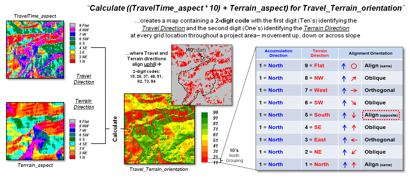
Figure 3. A 2-digit code is used
to identify all combinations of travel and terrain directions.
I realize the thought of “an aspect map of an abstract surface,” such
as a stepped accumulation surface might seem a bit uncomfortable and well
beyond traditional mapping; however it can provide very “real” and tremendously
useful information. Characterizing
directional movement is not only needed in backcountry emergency response but
crucial in effective timber harvest planning, wildfire propagation modeling,
pipeline routing and a myriad of other practical applications— such
out-of-the-box spatial reasoning approaches are what are driving geotechnology
to a whole new plane.
_____________________________
Author’s Note: for a detailed discussion of “stepped accumulation
surfaces,” see Topic 25, calculating Effective Distance and Connectivity in the
online book Beyond Mapping III posted at www.innovativegis.com/basis/MapAnalysis/.
Optimal Path Density is not all that Dense
(Conceptually)
(GeoWorld, January
2013)
The previous section addressed “Backcountry 911” that considers both
on- and off-road travel for emergency response.
Recall that the approach uses a stepped-accumulation cost surface
to estimate travel-time by truck, then all-terrain vehicle (ATV) and finally
hiking into areas too steep for ATVs.
The result is a map surface (formally termed an Accumulation
Surface) that identifies the minimum travel-time to reach all
accessible locations within a project area.
It is created by employing the “splash algorithm” to simulate movement
in an analogous manner to the concentric wave pattern propagating out from a
pebble tossed into a still pond. If the
conditions are the same, the effect is directly comparable to the uniform set
of ripples.
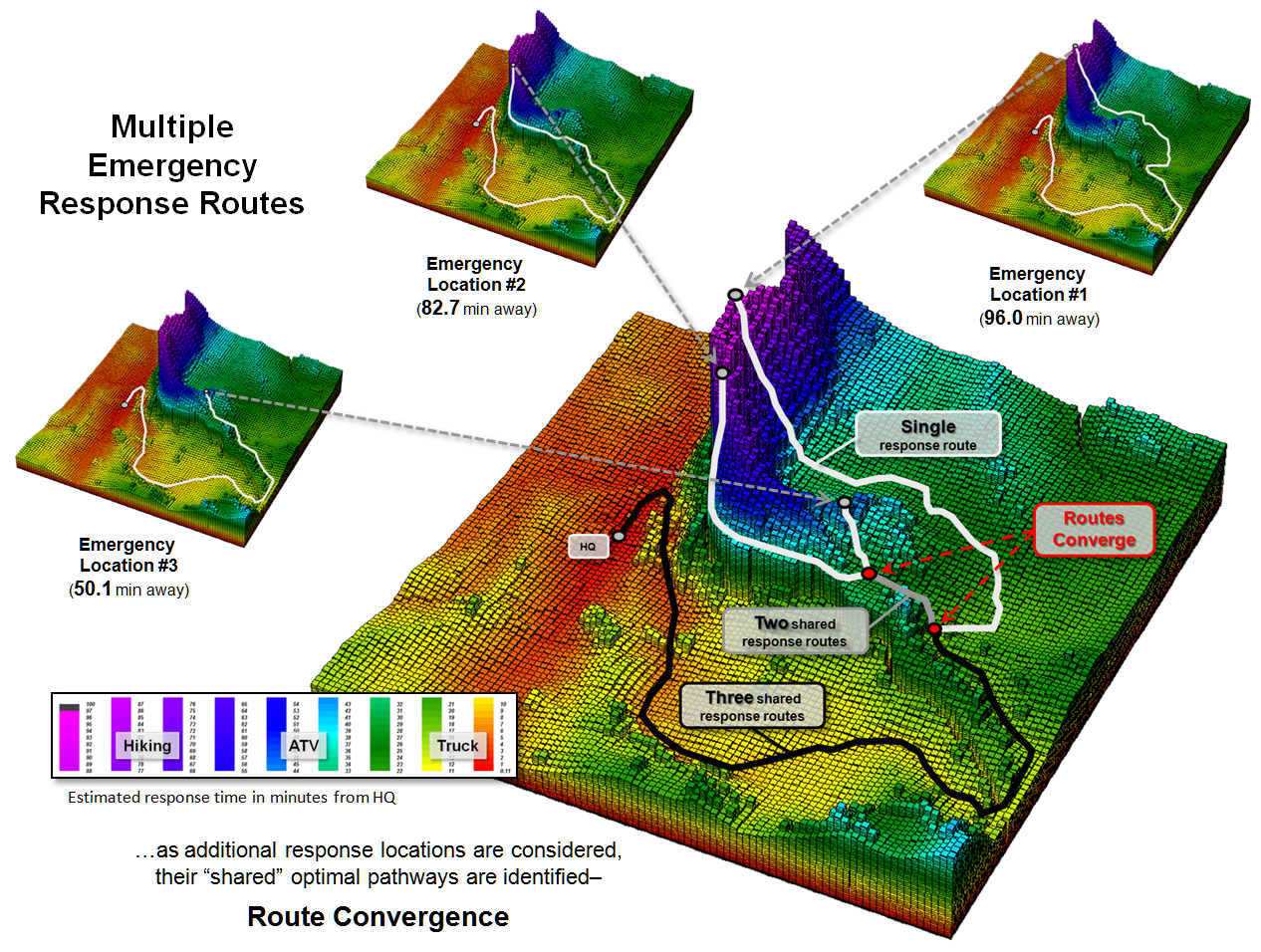
Figure 1. Multiple optimal paths
tend to converge to take advantage of “common access” routes over the
travel-time surface.
However as the wavefront encounters varying barriers to movement, the
concentric rings are distorted as they bend and wiggle around the barriers to
locate the shortest effective path. The
conditions at each grid location are evaluated to determine whether movement is
totally restricted (absolute barriers) or, if not, the relative difficulty of
the movement (relative barrier). The end
result is a map surface identifying the “shortest but not necessarily straight
line” distance from the starting location to all other locations in a project
area.
The emergency response surface shown in figure 1 identifies the minimum
travel-time via a combination of truck, ATV and hiking from headquarters (HQ)
to all other locations. Travel-time
increases with each wavefront step as a function of the relative difficulty of
movement that ultimately creates a warped bowl-like surface with the starting
location at the bottom (HQ= 0.0 minutes away).
The blue tones identify locations of very slow hiking conditions that result
in the “mountain” of increasing travel-time to the farthest away location
(Emergency Location #1= 96.0 minutes away).
The quickest route is rarely a straight line a crow might fly, but
bends and turns depending on the intervening conditions and how they affect
travel. The Optimal Path
(minimum accumulated travel-time route) from any location is identified as “the
steepest downhill path over the accumulated travel-time surface.” This pathway retraces the route that the
wavefront took as it moved away from the starting location while minimizing
travel-time at each step.
The small plots in the outer portion of Figure 1 identify the
individual optimal paths from three emergency locations. The larger center plot combines the three
routes to identify their convergence to shared pathways— grey= two paths and
black= all three paths.
The left side of figure 2 simulates responding to all accessible
locations in the project area. The
result is an “Optimal Path Density” surface that “counts the
number of optimal paths passing through each map location.” This surface identifies major confluence
areas analogous to water running off a landscape and channeling into gullies of
easiest flow. The light-colored areas represent travel-time “ridges” that
contain no or very few optimal paths.
The emergency response “gullies” shown as darker tones represent
off-road response corridors that service large portions of the
backcountry.
These “corridors of common access” are depicted as increasingly
darker tones that switch to red for locations servicing more than 256 potential
emergency response locations. Note that
9,853 locations of the 10,000 locations in the project area “drain” into the
headquarters location (the difference is the non-accessible flowing water locations).
This is powerful strategic planning information, as well as tactical
response routing for individual emergencies (backcountry 911 routing). For example, knowing where the major access
corridors intersect the road network can be used to identify candidate
locations for staging areas. The right
side of figure 2 identifies fifteen areas with high off-road access that
exceeds an average of sixteen optimal routes within a 1-cell reach from the
road. These “jumping off” points to the
major response corridors might be upgraded to include signage for volunteer
staging areas and improved roadside grading for emergency vehicle parking.
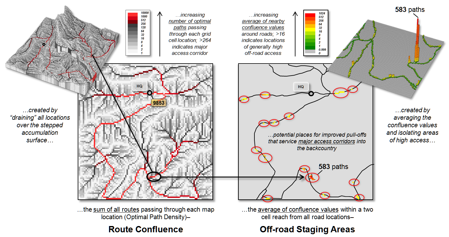
Figure 2. The sum of all optimal
paths passing through a location indicates its relative rating as a “corridor
of common access” for emergency response.
In many ways, GIS technology is “more different, than it is similar” to
traditional mapping and geo-query. It
moves mapping beyond descriptions of the precise placement of physical features
to prescriptions of new possibilities and perspectives of our geographic
surroundings— an Optimal Path Density surface is but one of many innovative
procedures in the new map analysis toolbox.
_____________________________
Author’s Note: a free-use poster and short papers on Backcountry
Emergency Response are posted at www.innovativegis.com/basis/Papers/Other/BackcountryER_poster/.
Assessing Wildfire Response (Part 1): Oneth by Land, Twoeth by Air
(GeoWorld, August
2011)
Wildfire initial attack generally takes three forms: helicopter
landing, helicopter rappelling or ground attack. Terrain and land cover conditions are used to
determine accessible areas and the relative initial attack travel-times for the
three response modes. This and next
month’s column describes GIS modeling considerations and procedures for
assessing and comparing alternative response travel-times.
The discussion is based on a recent U.S. Forest Service project
undertaken by Fire Program Solutions (see Author’s Notes). I was privileged to serve as a consultant for
the project that modeled the relative response times for all of the Forest
Service lands from the Rocky Mountains to the Pacific Ocean—at a 30m grid
resolution, that’s a lot of little squares.
Fortunately for me, all I needed to do was work on the prototype model,
leaving the heavy-lifting and “practical adjustments” to the extremely
competent GIS specialist, wildfire professionals and USFS helitack experts on
the team. The objectives of the project
were to model the response times for different initial attack modes and provide
summary maps, tables and recommendations for strategic planning and management
of wildfire response assets.
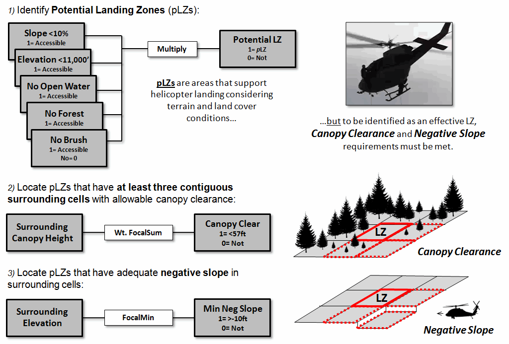
Figure 1. Generalized outline of a
grid-based model for identifying Potential Landing Zones (pLZs) that are
further evaluated for helicopter approach/departure considerations of Canopy
Clearance and Negative Slope.
The most challenging sub-model involved identifying helicopter landing
zones (see figure 1). A simple binary
suitability model is used to identify Potential Landing Zones (pLZs) by
assigning a map value of 1 to all accessible terrain (gentle slopes and
sub-alpine elevations) and land cover conditions (no open water, forest or tall
brush); with 0 assigned to inaccessible areas.
Multiplying the binary set of maps derives a binary map of pLZs with 1
identifying locations meeting all of the conditions (1*1*1*1*1= 1); 0 indicates
locations with at least one constraint.
Interior locations of large contiguous pLZs groupings make ideal
landing zones. However, edge locations
or small isolated pLZs clusters must be further evaluated for clear helicopter
approach/departure flight paths. At
least three contiguous cells surrounding a pLZ must have forest canopy of less
than 57 feet to insure adequate Canopy Clearance. In addition, it is desirable to have a Negative
Slope differential of at least 10 feet to aid landing and takeoff.
Two steps are required for evaluating canopy clearance (see figure
2). A reclassify operation is used to
calculate a binary map with canopy heights of 57 feet or less assigned a value
of 1; 0 for taller canopies. A
neighborhood operation (FocalSum in ArcGIS) is used to calculate the
number of clear canopy cells in the immediate vicinity of each pLZ cell (3x3
roving window). If all cells are clear,
a value of 9 will be assigned, indicating an interior location in a grouping of
pLZ cells.
For derived values less than 9, an edge location or isolated pLZ is
indicated. If there are more than four
surrounding cells with adequate clearance, there has to be at least three that
are contiguous and the pLZ is assigned a map value of 1 to indicate that there
is a clear approach/departure; 0 for locations with a sum of less than 4.
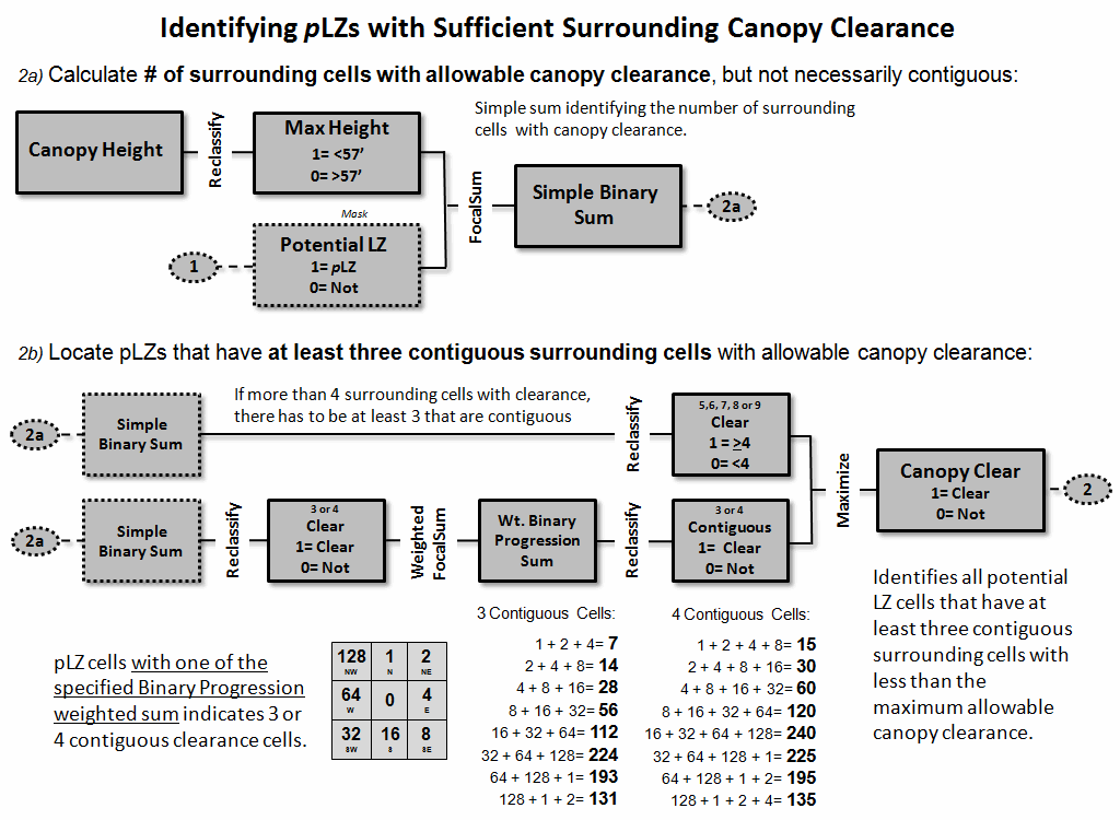
Figure 2. Procedure for
identifying pLZs with sufficient surrounding canopy clearance.
Derived values indicating 3 or 4 clear surrounding cells must be further
evaluated to determine if the cells are contiguous. First, locations with a simple binary sum of
3 or 4 are assigned 1; else= 0. A binary
progression weighted window—1,2,4,8,16,32,64,128—is used to generate a weighted
focal sum of the neighboring cells. The
weighted sum results in a unique value for all possible configurations of the
clear surrounding cells (see the lower portion of figure 2). For example, the only configuration that
results in a sum of 7 is the binary progression weights of 1+2+4 indicating
contiguous cells N,NE,E.
The weighted binary progression sums indicating contiguous cells are
then reclassified to 1; 0=else. Finally,
the minimum value for the “greater than 4 Clear” and “3 or 4 Clear” maps is
taken resulting in 1 for locations having sufficient contiguous canopy
clearance cells; else=0.
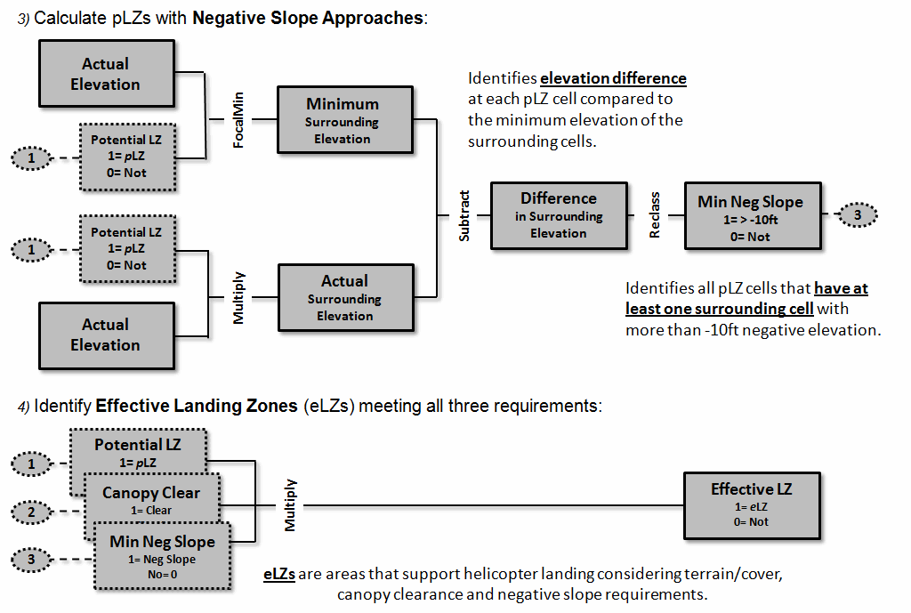
Figure 3. Procedures for
identifying pLZs with sufficient negative slope (top) and combining all three
considerations (bottom).
The top portion of figure 3 outlines the procedure for evaluating
sufficient negative slope by determining the difference between the minimum
surrounding elevation and each pLZ elevation.
If the difference is greater than 10 feet, a map value of 1 is assigned;
else= 0.
The final step multiplies the binary maps of Potential LZ, Canopy
Clearance and Minimum Negative Slope.
The result is a map of the Effective LZs as 1*1*1= 1 for locations
meeting all three criteria.
In the operational model, the negative slope requirement was dropped as
the client felt it was of marginal importance.
The next section describes the analysis approaches for identifying
ground response areas, helicopter rappelling zones and the translation of all
three response modes into travel-time estimates for comparison.
_____________________________
Author’s
Notes: For more information on
Fire Program Solutions and their wildfire projects contact Don Carlton, DCARLTON1@aol.com.
Assessing Wildfire Response (Part 2): Jumping Right into It
(GeoWorld,
September 2013)
The previous section noted that wildland fire initial attack generally
takes three forms: helicopter landing, helicopter rappelling or ground
attack as determined by terrain and land cover conditions (also “smoke-jumping”
but that’s a whole other story). The
earlier discussion described a spatial model developed by Fire Program
Solutions (see Author’s Notes) for identifying helicopter landing zones. The following discussion extends the analysis
to modeling and comparing the response times for the three different initial
attack modes for all locations within a project area.
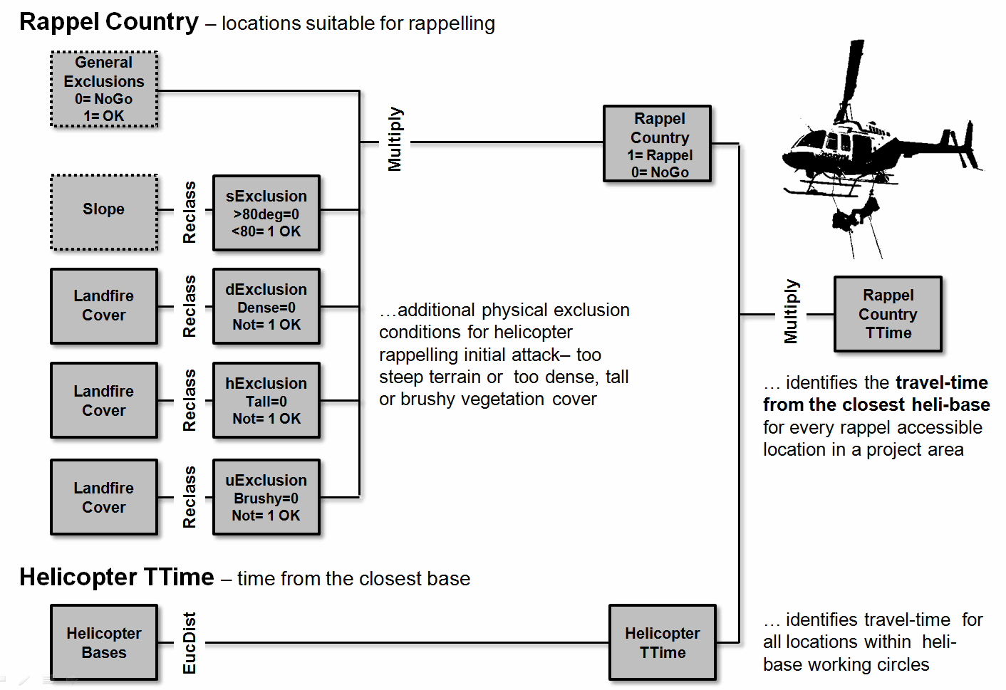
Figure 1. Major steps and
considerations in modeling wildfire Helicopter Rappel Attack travel-time.
Figure 1 identifies the major steps in determining “Rappel Country” …there
are some among us so heroic (crazy?) that they rappel out of a helicopter just
to get to a wildfire before the crowd.
Rappel country is defined as the areas where rappelling is the most
effective initial attack mode based on project assumptions. In addition to general exclusions (e.g., open
water, 10,000 foot altitude ceiling), rappelling must consider four other
highly variable physical exclusions— extremely steep terrain (>80 degrees),
very dense and/or tall forest canopies and dense tall brush. The simple binary model in the upper portion
of figure 1 is used to identify locations suitable for rappelling (1= OK; 0=
NoGo) where the fearless can jump from a hovering helicopter and slide down a
rope between the trees up to a couple of hundred feet to the ground.
The lower portion of the figure uses a simple distance calculation to
identify the travel-time within a 75 mile working circle about a helibase
assuming a defined airspeed, round trip fuel capacity and other defining
factors. By combining the binary map of
rappel country and the helicopter travel-time surface, an estimated travel-time
from the closest helibase to every Helicopter Rappelling Accessible location in
a project area is determined.
In a similar “binary multiplication” manner, the helicopter travel-time
to each Effective Landing Zone can be calculated. However, the landing crew must hike to a
wildland fire outside the landing zone.
This secondary travel is modeled in a manner similar to that used for
the off-road movement of the ground response model described below. The helicopter flight time to a landing zone
and the ground hiking time to the fire are combined for an overall travel-time
from the closest helibase to every Helicopter Landing Accessible location in a
project area.
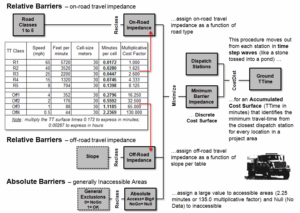
Figure 2. Major steps and
considerations in modeling wildfire Ground Attack travel-time.
Figure 2 outlines the major steps in modeling the combined on- and
off-road response time for a ground attack crew. On-road travel is determined by the typical
speed for different road types. The
calculations for deriving the travel-time to cross a 30m grid cell are shown in
the rows of the table for five classes of roads from major highways (R1) to
backwoods roads (R5). Note that the
slowest travel taking .1398 minute to traverse a backwoods road cell is over
eight times slower than the fastest (only .0172 min/cell).
Off-road travel is based on typical hiking rates under increasingly
steep terrain with the steepest class (2.2369 min/cell) being 130 times slower
than travel on a highway. In addition,
some locations form absolute barriers to ground movement (e.g., very steep slopes,
open water).
The three types of impedance are combined such that the minimum
friction/cost value is assigned to each location. A null value is assigned to locations with
absolute barriers. This composited
friction (termed a Discrete Cost Surface) is used to calculate the
effective distance for every location to the closest dispatch station. The procedure moves out from each station in time
step waves (like a stone tossed into a pond) that considers the
relative impedance as it propagates to generate an Accumulated Cost Surface
(TTime in minutes) identifying the minimum travel-time from the closest
initial dispatch location to every location in a project area (see Author’s
Notes).
The three separate travel-time surfaces can be compared to identify the
attack mode with the minimum response time (see figure 3) and the differential
times for alternative attack modes. In
operational situations, this information could be accessed for a fire’s
location and used in dispatch and tactical planning.
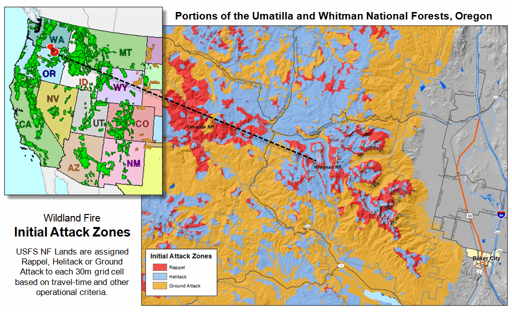
Figure 3. An example of a map of
the “best” initial attack mode for a fairly large area draped over a Google 3D
image.
In the “Rappel Country” project the information is used for strategic
planning of the arrangement of helibase locations with rappel initial attack
capabilities. Tabular summaries for
travel-time from existing helibases by terrain and land cover conditions were
generated. In addition, rearrangement of
helibase location and capabilities could be simulated and evaluated.
From a GIS perspective the project represents a noteworthy endeavor
involving advanced grid-based map analysis procedures over a large geographic
expanse from the Rocky Mountains to the Pacific Ocean that was completed in
less than four months by a small team of domain experts and GIS
specialists. The prototype analysis
originally developed was interactively refined, modified and enhanced by the
team and then applied over the expansive area.
As with most projects, database development and model
specification/parameterization formed the largest hurdles—the grid-based map
analysis component proved to be a “piece-of-cake” compared to nailing down the
requirements and slogging around in millions upon millions of geo-registered
30m cells …whew!
_____________________________
Author’s
Notes: For more information on
Fire Program Solutions, LLC and their wildfire projects contact Don Carlton, DCARLTON1@aol.com; for an in-depth
discussion of travel-time calculation, see the online book Beyond Modeling
III, Topic 25, Calculating Effective Distance, posted at www.innovativegis.com/Basis/MapAnalysis/Default.htm.
(Back to the Table of Contents)