|
Topic 8 – GIS
Modeling in Natural Resources |
GIS
Modeling book |
Harvesting
an Understanding of GIS Modeling — describes a prototype
model for assessing off-road access to forest areas
Extending
Forest Harvesting’s Reach — discusses a multiplicative
weighting method for model extension
E911 for the Backcountry — describes development of an on- and off-road travel-time
surface for emergency response
Extending Emergency Response Beyond the Lines — discusses basic model processing and
modifications for additional considerations
Comparing Emergency Response Alternatives — describes comparison procedures and route evaluation techniques
GIS’s Supporting Role in the Future of Natural Resources — discusses the influence of human
dimensions in natural resources and GIS technology’s role
Further Reading
— five additional sections
<Click here>
for a printer-friendly version of this
topic (.pdf).
(Back to the Table of Contents)
______________________________
Harvesting an Understanding of GIS Modeling
(GeoWorld, April 2010)
Vast regions of the Rocky
Mountains are under attack by mountain pine beetles and a blanket of brown is
covering many of the hillsides. Dead and
dying trees stretch to the horizon. In
five years there will be just sticks poking up and within twenty years the
forest floor will look like a game of “pick-up sticks” with a new forest poking
through.
It’s an ecological cycle,
but it is both aggravated by and aggravating to many of us who live and play in
the shadows of the mountains. Is there
something we can do to contain the spread and hasten the regenerative
cycle? One suggestion is to remove the
dead wood to speed forest health and convert it to useful products to
boot.
This appears attractive
but just knowing there are giga-tons of beetle-gnawed biomass awaiting “wood
utilization” solutions isn’t a fully actionable answer. What products are viable? Where and how much harvesting is appropriate?
These two basic questions
captured the attention of combined graduate project teams at the University of
Denver. A “capstone MBA” team focused on
the business case while a “GIS modeling” team focused on the geographic
considerations. Their joint experience
in identifying, describing and evaluating potential solutions provided an
opportunity to get their heads around a complex issue requiring integration of
spatial and non-spatial analysis, both at a macro state-wide level and a micro
local level. The experience also
provides a springboard for a short Beyond Mapping series on GIS modeling (scar
tissue and all).
Our outside collaborators
(a non-profit organization and a large energy company) narrowed the
investigation to biomass for augmentation of base-load electric energy
generation—first lesson, always heed the client’s interests. This assumption narrows the macro
considerations as haul distances from a plant are critical. Considering mountainous travel, buffering to
a simple geographic distance is insufficient and travel-time zones were
recommended—second lesson, clients love the on-road travel-time concept.
The concept of modeling
off-road access, on the other hand, is a bit harder to appreciate. It was decided that a micro level “proof-of-concept
prototype model” for assessing forest access would be developed. Figure 1 depicts the map variables and basic
approach taken for a hypothetical demonstration area—third lesson, never use
real data for a prototype model if you want clients to concentrate on model
logic.
The first phase of the
basic model determines Availability of lands for harvesting
activity. Legal concerns, such as
ownership, stream buffers and sensitive areas must be identified and
unavailable lands removed from further consideration. In addition, physical conditions can become
“absolute barriers,” such as steep slopes beyond the operating range of
equipment. A second phase characterizes
the relative Access of available lands by considering intervening
conditions as “relative barriers,” such as increasing slope in operable areas
increases costs of harvesting.
It is important not to
“over-drive” the purpose of a Prototype Model as a mechanism for demonstrating
a viable approach and stimulating discussion—fourth lesson, “keep it simple
stupid (KISS)” to lock a client’s focus on model approach and logic. Anticipated refinements should be reserved
for a “Further Considerations” section in the presentation describing the
prototype model.
If model refinement
accompanies prototype development, there isn’t a need for a prototype.
But that is the bane of a “waterfall approach” to GIS modeling. You can easily drown by jumping off the edge
at the onset; whereas calmly walking into the pool with your client engages and
involves them, as well as bounds a
manageable first cut of the approach and logic … baby steps with a
client, not a top-down GIS’er solution out of the box. Fifth lesson—there
is a sweet spot along a client’s perception of a model from a Black box of
confusion to Pandora’s box of terror.
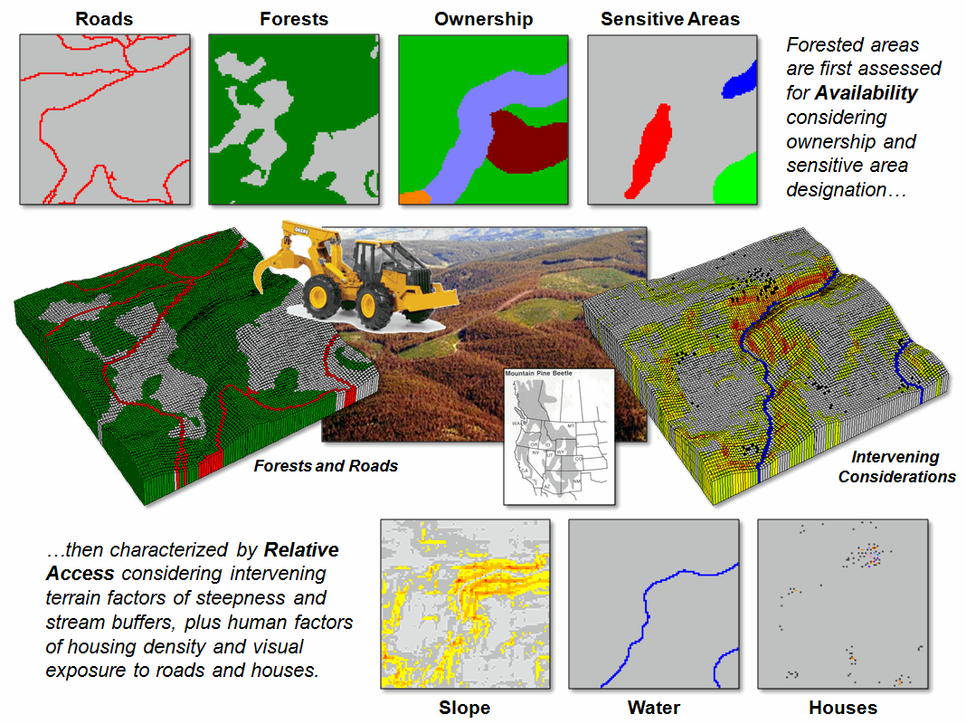
Figure 1.
Relative harvesting access is determined by availability of forest lands
as modified by intervening conditions.
Figure 2 contains a
flowchart of model logic for the basic Availability/Access prototype
model. Only four base maps and ten
commands are involved in a demonstrative first cut. A Slope map is used to derive slope impedance
where ranges of steepness are assigned 1 (most preferred)= 0-10%, 2= 10-20%, 4=
20-30% 7 (seven times less preferred)= 30-40% and 0 (unavailable)=
>40%.
The other maps of
Ownership, Water and Sensitive Areas are used to derive binary maps where 1=
available and 0= unavailable lands. The
final step calculates the acreage of accessible forests within each watershed.
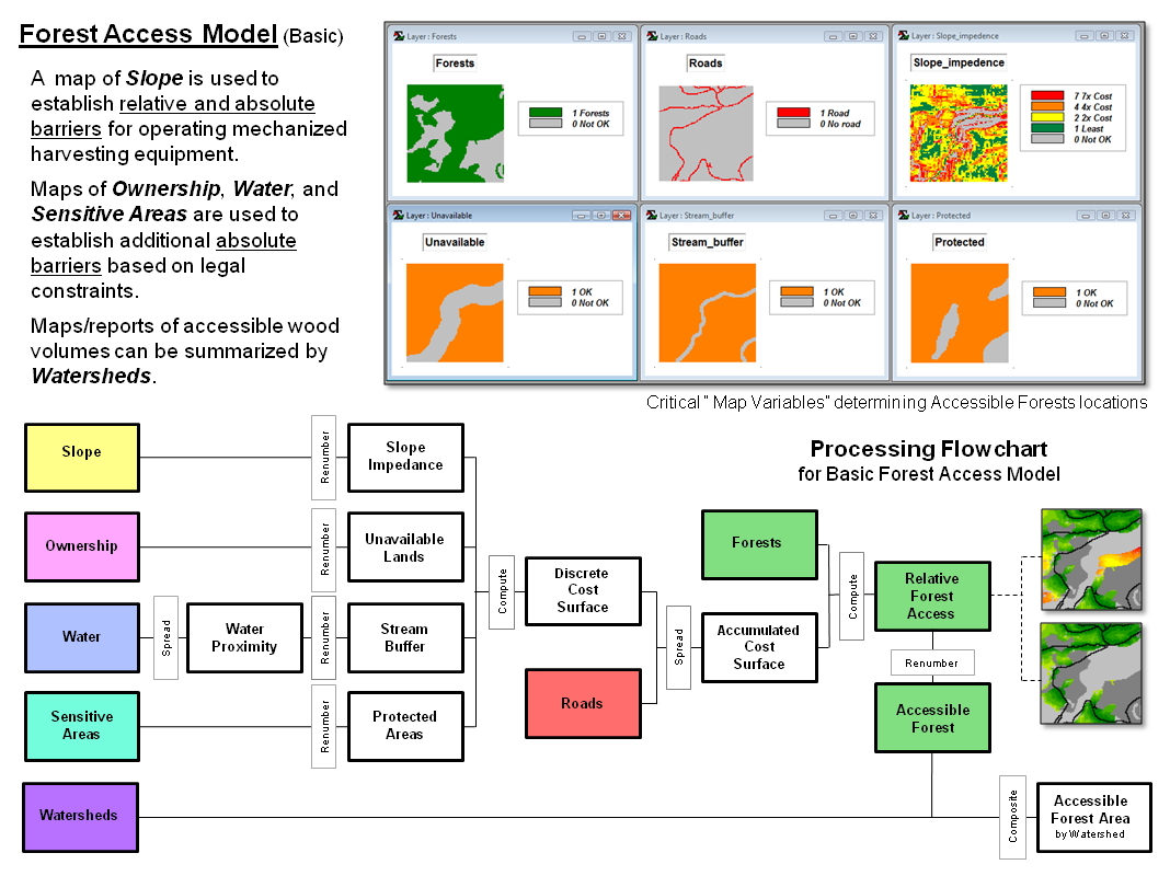
Figure 2. Flowchart of the basic model involves four
base maps and ten processing commands.
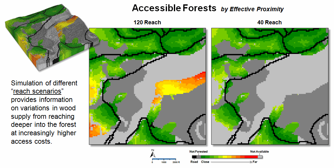
Figure 3. Different effective “reaches” into the
accessible forested areas can be generated to simulate varying budget
sensitivities.
The four calibrated maps
are multiplied for a Discrete Cost Surface that contains a zero for unavailable
lands (any 0 in the map stack sends that location to 0) and the relative
“friction values” based on terrain steepness are preserved for available areas
(1 * 1* 1 * friction value retains that value).
In turn, this map is used to generate the relative access map using a
“Least Cost” approach that will be discussed in next month’s column that “lifts
the hood” on technical considerations (see Author’s note).
Figure 3 provides an
early peek at some of the output generated by the basic Forest Access
model. The left inset shows the relative
access values for all of the available forested areas with warmer tones
indicating a long harvesting reach into the woods; light grey, unavailable and
dark grey, non-forested. A user can
conjure up different “reach” scenarios defining accessible forests as a means
to understand the spatial relationships from grabbing just the “low hanging
economic fruit (…err, I mean wood)” that is easily accessed (right inset), to
increasingly aggressive plunges deeper into the woods at increasingly higher
access costs.
Also, consideration of
human concerns, such as housing density and visual exposure, might affect a
practical assessment of the access reach.
Finally, locating suitable staging areas (termed “Landings”) for wood
collection and the delineation of the forest areas they serve (termed
“Timbersheds”) provide even more fodder for next couple of columns.
_____________________________
Author’s Note: For more discussion on effective distance and connectivity, see
Beyond Mapping Compilation Series, book III, Topic 4, “Calculating Effective
Distance” and book IV, Topic 2, “Extending Effective Distance Procedures”
posted at www.innovativegis.com.
Extending
Forest Harvesting’s Reach
(GeoWorld, May 2010)
The previous section
described a basic spatial model for determining relative harvesting
availability and accessibility of beetle-killed forests for harvesting. The prototype model was developed by “capstone
MBA” and “GIS modeling” graduate teams at the University of Denver. A non-profit organization and a large energy
company served as outside collaborators and narrowed the focus to the
extraction of biomass for base-load electrical energy generation.
State-wide analysis
involving on-road travel was proposed for assessing hauling distances of wood
chips to power plants where the resource would be further refined and mixed
with coal. Adjusting for mountainous
travel along the road network, some beetle-kill areas simply are too far from a
plant for consideration.
Local level analysis
involving off-road harvesting is considerably more complex. In summary, this processing determines the
relative accessibility from the landings into the forest considering a variety
of terrain, ownership and environmental considerations. Adjusting for off-road access, some
beetle-kill areas are unavailable or effectively too far from roads for
harvesting.
The Basic Access Model
outlined in the top portion of figure 1 demonstrates the types of factors that
can be considered in assessing off-road access.
The processing first identifies absolute barriers to harvesting
based on ownership, environmentally sensitive areas, water buffers and terrain
that is too steep for equipment to operate.
These factors are represented as binary map layers with 1= available and
0= unavailable for harvesting activity.
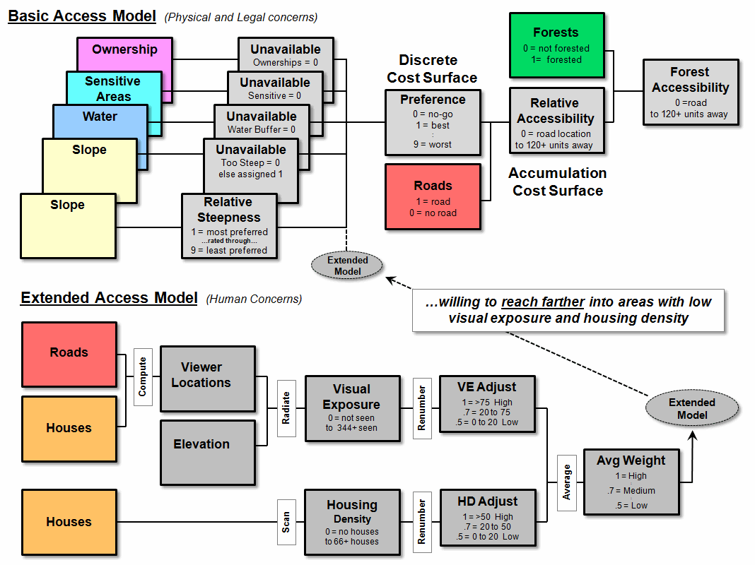
Figure 1. The
Extended Access Model develops a multiplicative weighting factor based on
housing density and visual exposure of potential harvesting areas.
Relative barriers to forest access are rated from 1= most preferred
to 9= least preferred. In the prototype
model, slopes within the harvesting equipment operating range are used to
demonstrate relative barriers with increasingly steeper slopes becoming less
and less desirable. Multiplying the
stack of map layers identifying absolute and relative barriers results in an
overall preference surface for harvesting with values from 0 (no-go), to 1
(best) through 9 (worst). The final step
uses grid-based effective distance techniques to determine the relative
accessibility of available forested areas from roads (see author’s note).
As an extension to the
basic model, human concerns for minimizing visual exposure and housing density
are outlined in the lower portion of figure 1.
The procedure first derives a visual exposure density surface
identifying the number of times each location is seen from houses and roads and
then calibrates the exposure from .5 (low exposure) through 1.0 (high
exposure). Similarly, a housing density
surface identifying the number of houses within a half mile radius was
calibrated from .5 (low density) to 1.0 (high density). The two adjusted maps are averaged for an
overall weighting factor for each map location.
When the multiplicative
weight is applied to the preference map stack, it improves (lowers) preference
ratings in areas with low visual exposure and housing density, while retaining
the basic ratings in areas of high visual exposure and housing density. The effect on the model is to favor reaching
farther into available forested areas in locations that are less
contentious.
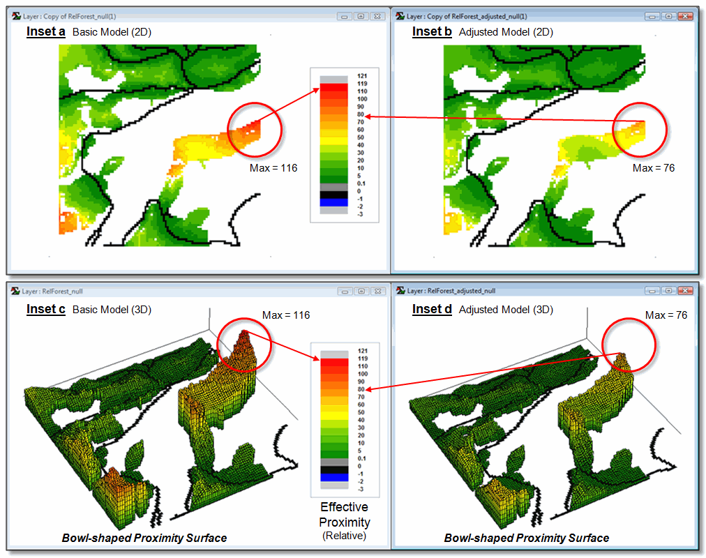
Figure 2. Comparison of Basic and Extended model
results.
Figure 2 compares the
results with the left side of the figure tracking the results of Basic Model
and the right side tracking the results of the Extended Model that favors
harvesting in areas of low human impact.
The effective distance to the farthest available forest location is
reduced by a third from 116 to 76. The
3D plots on the bottom of the figure (insets c and d) depict the results as
bowl-shaped accumulation surfaces with the lowest value of 0 “cells away” from
the road in the lower center portion of the project area. Note the considerable easing (lower values;
flattening of the surface) of the relative proximity at the circled remote
location.
Figure 3 illustrates a
couple of techniques for summarizing related map information using a binary map
of accessible forest areas. A
region-wide (zonal) overlay operation can be used to “count” the total number
of acres of accessible forest in each of the three watersheds (e.g., 374 aces
of accessible forest in Watershed 3).
Also, by simply multiplying the binary map times the vegetation map
identifies the vegetation type and area for all of the accessible forest
locations (e.g., 964 acres of accessible Lodgepole pine).
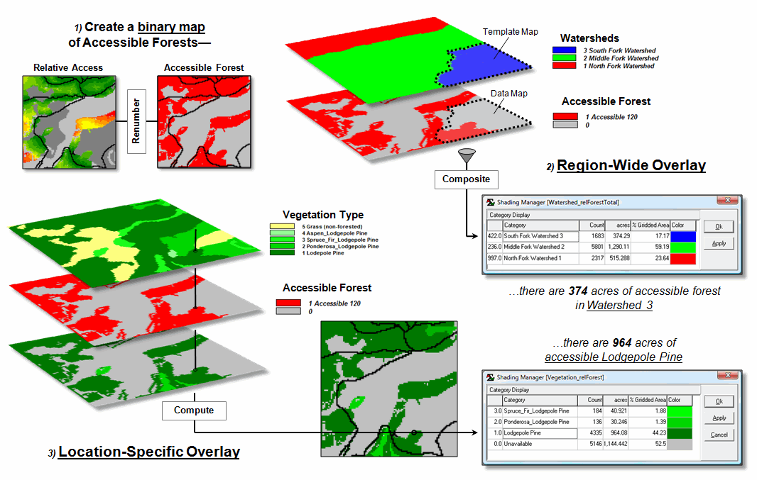
Figure 3. D. Summarizing accessible forest areas by
watersheds and vegetation type.
The ability to repackage
all beetle-kill areas into those meeting harvesting availability and access
requirements is critical. Just knowing
that there are giga-tons of biomass out there isn’t sufficient until they are
mapped within a comprehensive decision-making context. Additional extensions include procedures for
determining the best set of staging areas, termed “landings,” and the
characterization of the potential wood chip supply within each of their
corresponding “timbersheds” (see Author’s Notes).
The next three sections
consider on- and off-road travel for backcountry emergency response. The basic approach using effective distance
is similar to harvesting access except the identification and response time for
the optimal route (minimum travel-time) by truck, ATV and hiking between two
locations is the goal.
_____________________________
Author’s Note: For a discussion on identifying and
characterizing “Timbersheds” see Further Online Reading section 1, “A Twelve-step Program for
Recovery from Flaky Forest Formulations”at the
end of this topic.
E911 for the Backcountry
(GeoWorld, July 2010)
One of the most important
applications of geotechnology has been Enhanced 911 (E911) location technology
that enables emergency services to receive the geographic position of a mobile
phone. The geographic position is
automatically geo-coded to a street address and routing software is used to
identify an optimal path for emergency response. But what happens if the call that “I’ve
fallen and can’t get up” comes from a backcountry location miles from a
road? The closest road location “as the
crow flies” is rarely the quickest route in mountainous terrain.
A continuous space
solution is a bit more complex than traditional network analysis as the
relative and absolute barriers for emergency response are scattered about the
landscape. In addition, the intervening
conditions affect modes of travel differently.
For example, an emergency response vehicle can move rapidly along the
backcountry roads, and then all terrain vehicles (ATV) can be employed off the
roads. But ATVs cannot operate under
extremely steep and rugged conditions where hiking becomes necessary.
The left side of figure 1
illustrates the on-road portion of a travel-time (TT) surface from headquarters
along secondary backcountry roads. The
grid-based solution uses friction values for each grid cell in a manner
analogous to road segment vectors in network analysis. The difference being that each grid cell is
calibrated for the time it takes to cross it (0.10 minute in this simplified
example).
The result is an estimate
of the travel-time to reach any road location.
Note that the on-road surface forms a rollercoaster shape with the
lowest point at the headquarters (TT = 0 minutes away) and progressively
increases to the farthest away location (TT = 26.5 minutes). If there are two or more headquarters, there
would be multiple “bottoms” and the surface would form ridges at the
equidistance locations in terms of travel-time—each road location assigned a
value indicating time to reach it from the closest headquarters.
Figure 1. On-road emergency response travel-time.
The lower-right portion
of figure 1 shows the calibrations for on-road travel by truck and off-road
travel by ATV and hiking as a function of terrain steepness and recognition of
rivers as absolute barriers to surface travel.
The programming trick at this point is to use the accumulated on-road
travel-time for each road location as the starting TT for continued movement
off-road. For example, the off-road
locations around the farthest away road location starts “counting” at
26.5, thereby carrying
forward the on-road travel time to get to off-road locations. As the algorithm proceeds it notes the on-
and off-road travel-time to each ATV accessible location and retains the
minimum time (shortest TT).
Figure 2 identifies the
shortest combined on- and off-road travel-times. Note that the emergency response solution
forms a bowl-like surface with the headquarters as the lowest point and the
road proximities forming “valleys” of quick access. The sides of the valleys indicate ATV
off-road travel with steeper rises for areas of steeper terrain slopes (slower
movement; higher TT accumulation). The
farthest away location accessible by truck and then ATV is 52.1 minutes.
Figure 2. On-road plus off-road travel-time using
ATV under operable terrain conditions.
The grey areas in the
figure indicate locations that are too steep for ATV travel, particularly
apparent in the steep canyon area (lower left insert with warmer tones of Slope
draped over the Elevation surface). The
sharp “escarpment-like” feature in the center of the response surface is caused
by the absolute barrier effect of the river—shorter/easier easier access from
roads west of the river.
Figure 3 completes the
emergency response surface by accounting for hiking time from where the wave
front of the accumulated travel-time by truck and ATV stopped. Note the very steep rise in the surface (blue
tones) resulting from the slow movement in the rugged and steep slopes of the
canyon area. The farthest away location
accessible by truck, then ATV and hiking is estimated at 96.0 minutes.
The lower-left insert
shows the emergency response values draped over the Elevation surface. Note that the least accessible areas occur on
the southern side of the steep canyon.
The optimal (quickest) path from headquarters to the farthest location
is indicated—that is within the assumptions and calibration of the model.

Figure 3. On-road plus off-road travel-time by ATV
and then hiking under extreme terrain conditions.
The bottom line of all
this discussion is that GIS modeling can extend emergency response planning
“beyond the lines” of a fixed road network—an important spatial reasoning point
for GIS’ers and non-GIS’ing resource managers alike.
_____________________________
Author’s Note: See www.innovativegis.com/basis/MapAnalysis/Topic29/EmergencyResponse.htm
for an animated slide set illustrating the incremental propagation of the
travel-time wave front considering on- and off-road travel and materials for a
“hands-on” exercise in deriving continuous space emergency response surfaces.
Extending Emergency
Response Beyond the Lines
(GeoWorld, August 2010)
The previous section
described a basic GIS model for backcountry emergency response considering both
on- and off-road travel. The process
used grid-based map analysis techniques that consider the spatial arrangement
of absolute barriers (not passable) and relative barriers (passable with
varying ease) that impede emergency response throughout continuous geographic
space.
While the processing
approach is conceptually similar to Network Analysis, movement is not
constrained to a linear network of roads represented as a series of irregular
line segments but can consider travel throughout geographic space represented
as a set of uniform grid cells. The
model assumes that the response team first travels by truck along existing
roads, then off-loads their all-terrain vehicles (ATV) for travel away from the
roads until open water or steep slopes are encountered. From there the team must proceed on
foot. The result of the model is a
travel-time map surface with an estimated minimum response time assigned to
each map location in a project area.
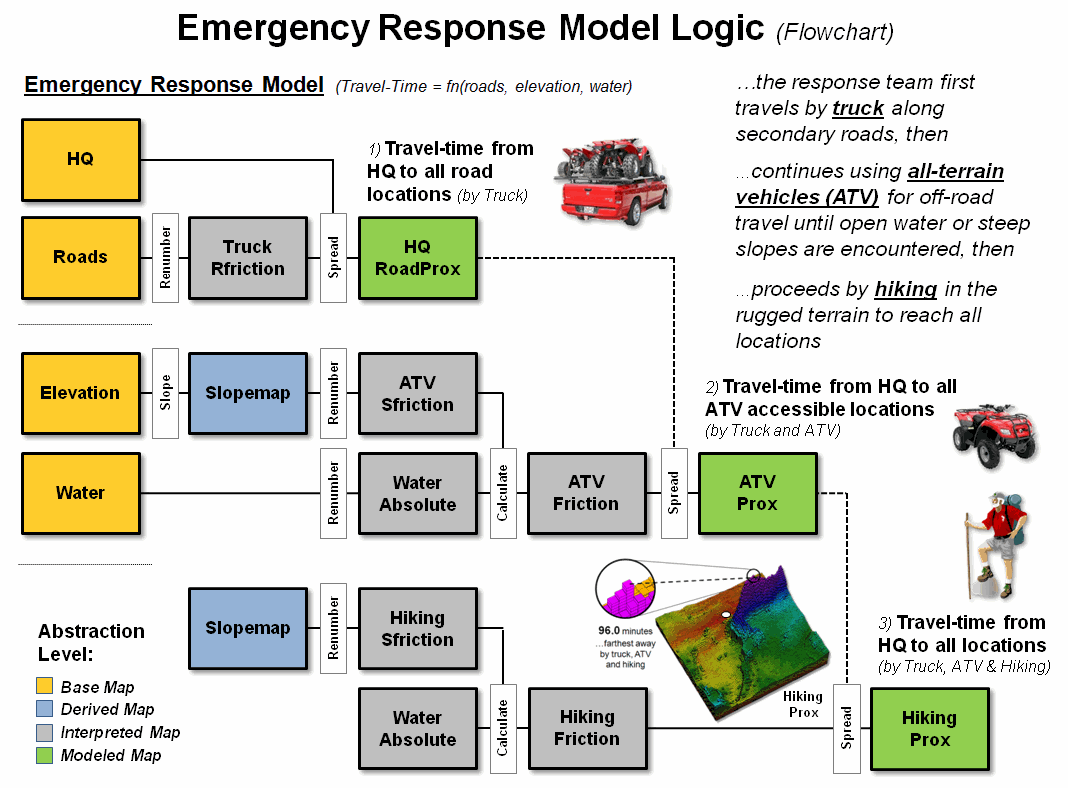
Figure 1. Flowchart of map analysis processing to
establish emergency response time to any location within a project area.
Last section’s discussion
described the key conceptual considerations and results of the three stages of
backcountry emergency response model—truck, ATV and hiking movement. The most notable points were that movement
proceeds as ever increasing waves emanating from a staring location that are
guided by absolute/relative barriers and
results in a continuous travel-time map (bowl-like 3D surface).
Figure 1 outlines the
processing as a flowchart. Boxes
represent map layers and lines represent analysis tools (MapCalc commands are
indicated). The flowchart is organized
with columns characterizing “analysis levels” proceeding from Base maps
(existing data), to Derived maps, to Interpreted maps, to Modeled map
solutions. The progression reflects a
gradient of abstraction from “fact-based” (physical) characterization of the
landscape involving Base and Derived maps, through increasingly more
“judgment-based” (conceptual) characterizations involving Interpreted and
Modeled maps expressing spatial relationships within the context of a problem.
The row groupings represent
“criteria considerations” used in solving a spatial problem. In this case, the processing first considers
truck travel along the roads then extends the movement off-road by ATV travel
and finally hiking into the areas that are inaccessible by ATV. The off-road movement is guided by open water
(absolute barrier for both ATV and hiking) and terrain steepness (relative
barrier for both ATV and hiking and absolute barrier for ATV in very steep
slopes).
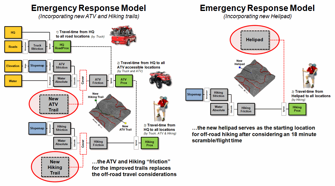
Figure 2. Extended response models for new trails
(left) and helipad (right).
Figure 2 identifies
modifications to the model considering construction of new ATV and hiking trails
and a helipad. The left side of the
figure updates the ATV and hiking “friction” maps with lower travel-time values
for the trails over the unimproved off-road travel impedances. The hiking trail includes a foot bridge at
the head of the canyon that crosses the river.
The revised friction values (ATV trail = 0.15 minutes; hiking trail =
0.5 minutes) directly replace the old values using a single command and the
model is re-executed.
In the case of the new
helipad (right side of the figure) the hiking submodel is used but with a new
starting location that assumes an 18 minute scramble/flight time to reach the
location.
The bottom portion of
figure 3 shows the three emergency response surfaces. Visual inspection shows considerable
differences in the estimated response time for the area east of the river.
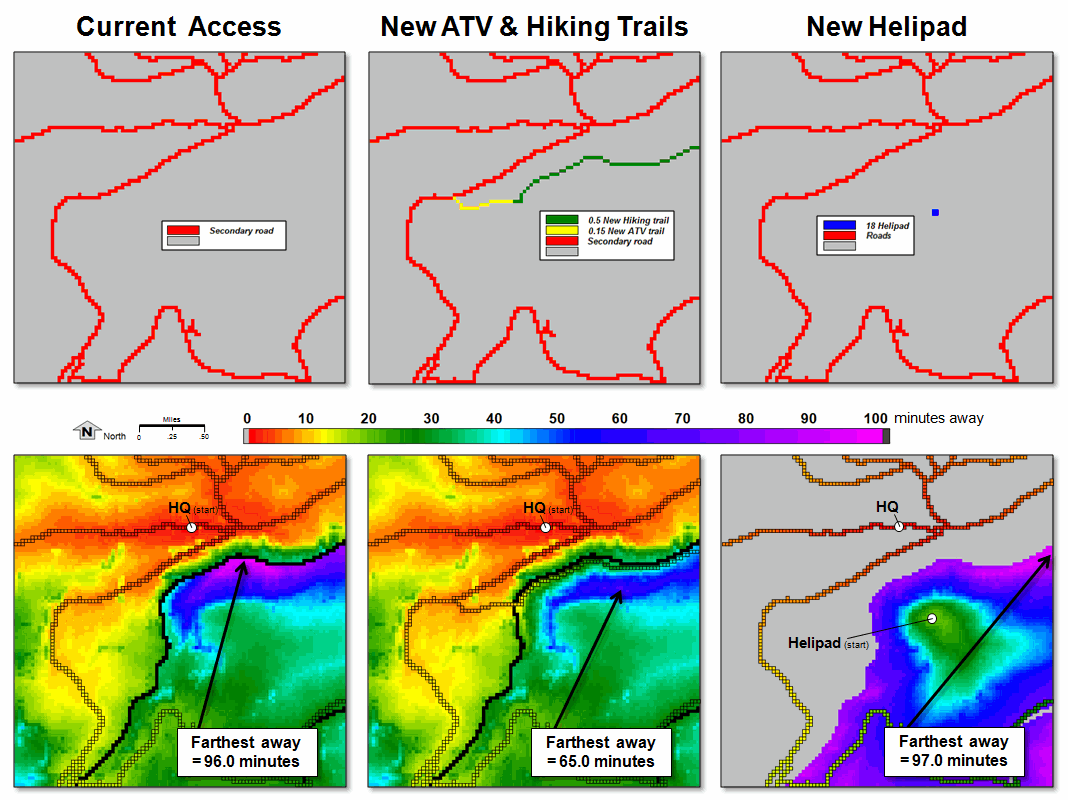
Figure 3. Emergency response surfaces for the
current situation, additional trails and helipad.
Current access requires
truck travel across the bridge over the river in the extreme SW portion of the
project area. Construction of the new
trails provides quick ATV access to the foot bridge then easy hiking on the
improved trail along the eastern edge of the river for faster response times on
the east side of the canyon (light blue).
Construction of the new helipad greatly improves response time for the
upper portions of the east side of the canyon.
The next section’s discussion
focuses on quantifying the changes in response time and developing routing
solutions that indicate the type of travel (truck, ATV, hiking, helicopter) for
segments along the optimal path to any location.
Comparing Emergency Response Alternatives
(GeoWorld, September 2010)
The last couple of
sections described a simplified backcountry emergency response model
considering both on- and off-road travel and then extended the discussion by
simulating two alternative planning scenarios—the introduction of a new
ATV/Hiking trail and a Helipad. The
conceptual framework, procedures and considerations in developing the
alternative scenarios were the focus.
This section’s focus is on comparison procedures and route evaluation
techniques.
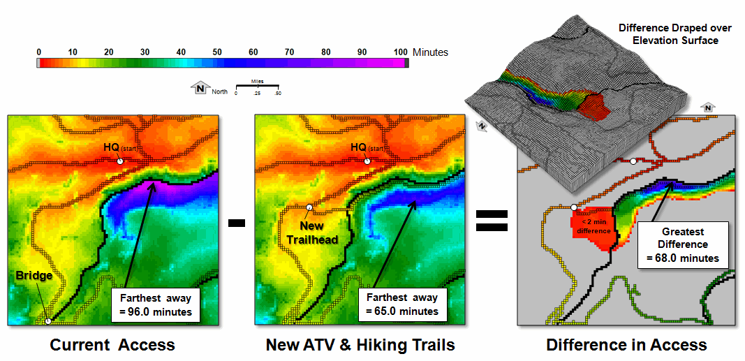
Figure 1. Subtracting two travel-time surfaces
determines the relative advantage at every location in a project area.
The left side of figure 1
depicts the minimum expected travel-time from headquarters to all locations
within a project area under current conditions.
The river in the center (black) acts as an absolute barrier that forces
all travel to the southeastern portion across a bridge in the extreme
southwest. This makes the farthest away
location more than an hour and a half from the headquarters, although it is
less than half a mile away “as the crow flies.”
The inset in the center
of the figure locates a proposed new ATV/Hiking trail. The first segment of from the road to the
river enables ATV travel. A light
suspension bridge crosses the river to provide hiking access to an improved
trail along the southern side of the canyon.
While the trail is
justified primarily for increasing recreation potential within the canyon, it
has considerable impact on emergency response in the canyon. Note the introduction of the green and light
blue tones along the river that indicate response times of about half an hour
as compared to more than an hour and a half (purple) currently required.
The right side of figure
1 shows the difference in travel-time under current conditions and the proposed
new trail. This is accomplished by
simply subtracting the two maps—where 0 = unchanged response times (light
grey), values = difference in the response times (red through blue tones). The red area between the road and the suspension
bridge notes that ATV access is slightly improved (less than 2 minutes
difference) with the introduction of the new trail. The greens and blues show considerable
improvement in response time with a maximum difference of 68.0 minutes.
Draping the result over
the elevation surface shows that the south side of the canyon bottom is best
serviced via the new trail. The more
important, non-intuitive information is the dividing line of best access
approach (red line) halfway up the southern side of the canyon. Locations nearer the top of the canyon are
best accessed via the current truck/ATV/Hiking utilizing the southern bridge.
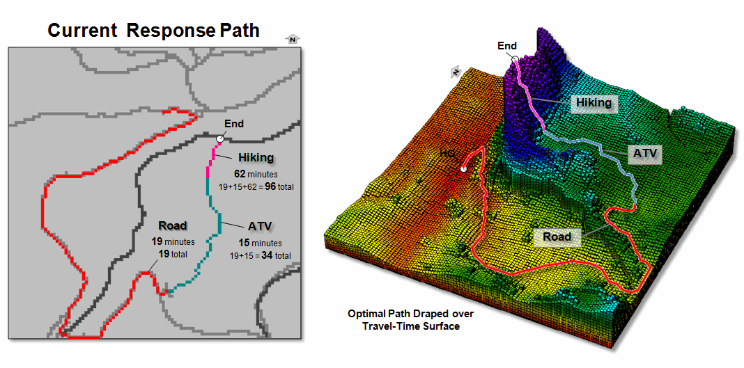
Figure 2. The optimal path is identified as the
steepest downhill route over a travel-time surface. (see Author’s Note)
Figure 2 extends the
analysis to characterize the optimal path for the most remote location under
current conditions. The first segment (red)
routes the truck along the road for approximately 19 minutes to an old logging
landing. The ATV’s are unloaded and
precede off-road (cyan) toward the northeast for an additional 15 minutes (19 +
15= 34 minutes total). Note the route’s
“bend” to the east to avoid the sharply increased travel-time in the rugged
terrain along the west canyon rim as depicted in the travel-time surface.
Once the southern side of
the canyon becomes too steep for the ATVs, the rescue team hikes the final
segment of 62 minutes (violet) for an estimated total elapsed time of 96
minutes (19 + 15 + 62 = 96). A digitized
routing file can be uploaded to a handheld GPS unit to assist off-road
navigation and real-time coordinates can be sent back to headquarters for
monitoring the team’s progress—much like commonplace network
navigation/tracking systems in cars and trucks, except on- and off-road
movement is considered.
The backbone of the
backcountry emergency response model is the derivation of the travel-time
surface (right side of figure 2). It is
“calculated once and used many” as any location can be entered and the steepest
downhill path over the surface identifies the best response route from
headquarters—including Truck, ATV and Hiking segments with their estimated
lapsed times and progressive coordinates.
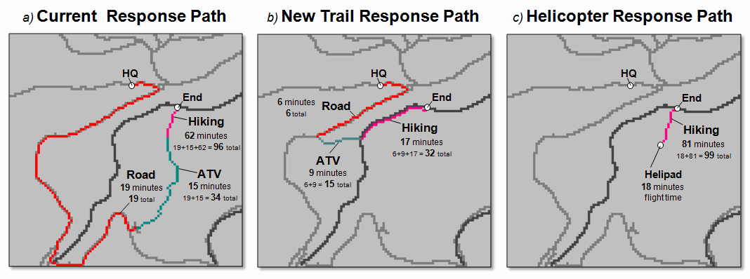
Figure 3. Comparison of emergency response routes to
a remote location under alternative scenarios.
In addition, alternate
scenarios can be modeled for different conditions, such as seasons, or proposed
projects. For example, figure 3 shows
three response routes to the same remote location—considering a) current conditions,
b) new trail and c) new helipad. In this
case, the response is much quicker for the new trail route versus either the
current or helipad alternatives.
It is important to note
that the validity of any spatial model is dependent on the quality of the
underlying data layers and the robustness of the model—garbage in (as well as
garbled throughput) is garbage out. In
this case, the model only considers one absolute barrier to movement (water)
and one relative barrier (slope) making it far too simplistic for operational
use. While it is useful for introducing
the concept, but considerable interaction between domain experts and GIS
specialists is needed to advance the idea into a full-fledged application …any
takers out there?
_____________________________
Author’s Note: See Beyond Mapping Compilation Series, book
III, Further Reading section 6, “Derive
and Use Hiking-Time Maps for Off-Road Travel” posted at www.innovativegis.com for a more
detailed discussion on deriving off-road travel-time surfaces and establishing
optimal paths.
GIS’s Supporting Role in the Future of Natural Resources
(GeoWorld, December 2010)
My completely charming
wife recently made a thought-provoking presentation entitled “Human Dimensions:
From Backstage to Front and Center” for a seminar series on Decades of Change
in Ecological Research at Colorado State University. In the talk she made reference that in 1970s
individual disciplinary scientists controlled the podium of discussion, and
social science, its issues and human dimensions, were primarily back stage in
natural resource research, planning and management (left side of figure 1).
In the 1980s, the podium
became a “team table” with a diversity of disciplines collaboratively engaged
in science-based discussion for assessing management options. The discussion around the table was expanded
to include social science’s theories and understandings of human values,
attitudes and behaviors.
During the 1990s, the
team table expanded further to a room full of “banquet tables” containing a
broad diversity of interests promoting direct and active engagement of
scientists, managers, stakeholders and representative publics in the
conversation. The interaction was
space/time bound to scheduled meetings, representative input, organized
discussion and manual flip chart documentation.
What dramatically changed
over the years is the role of human dimensions in addressing natural resource
issues from its early “back stage” position to a “front and center” involvement
and increasingly active voice.
Today and into the
future, Social Acceptability has fully joined Ecosystem
Sustainability and Economic Viability as a critical third filter
needed for successful decision-making (figure 2). Like a three-legged stool, removal of any of
the legs results in an unstable condition and the likelihood of failed
decisions.
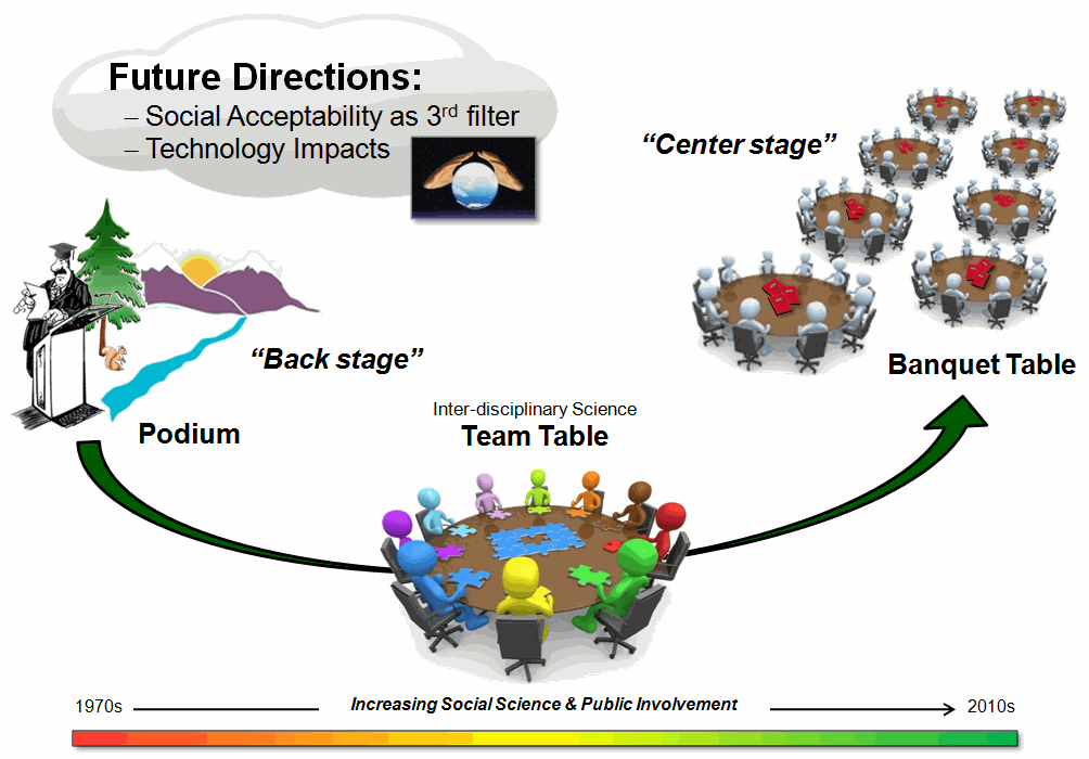
Figure 1. Social science and human dimensions in
natural resources have moved from back stage to front and center.
Joining social
acceptability as a significant factor impacting the future of natural resources
is the changing capabilities and roles of technology— with geotechnology poised
to play a key supporting role.
Spatially-enabled Social Networking concepts, such as “community
collaborative mapping,” “participatory GIS,” “user generated content” and the
“spatial tweet” will be the shared futures of social science, natural resources
and geotechnology.
To a large extent, GIS
technology had a fairly slow start in natural resources as practical
application got mired in the forest mensuration and mapping units within most
NR organizations— data first, utility later.
While innovative research projects demonstrated new ways of doing
business with spatial data, the data-centric perspective of the specialists
(mapping and geo-query) dominated the analysis-centric needs of the managers,
policy and decision makers (spatial reasoning and modeling).
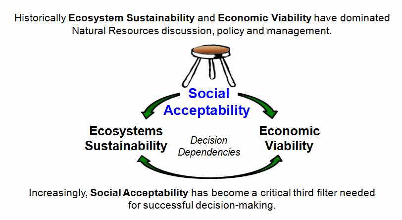
Figure 2. Social acceptability of plans and policy
has become an important third filter in natural resources management.
But with the growing
voice of human dimensions in natural resources there appears to be a plot twist
in the works. Maps are being viewed less
and less as static wall hangings depicting “where is what” and more as
dynamic spatial expressions of “why, so what and what if…” within the
context of alternative management and policy options.
That brings us to one of
the hottest new things in computing… “crowdsourcing.” In case some of you (most?) might not be
aware of this new field, a thumbnail sketch with a bit of discussion seems in
order (figure 3). Crowdsourcing
is a term that mashes the words "crowd" and "outsourcing"
to describe the act of taking tasks traditionally performed by a team of
in-house or outsourced specialists, and outsourcing the tasks to the community
through an ‘open call’ to a large group of people (the crowd) asking for their
input (Wikipedia).
For example, the public
may be invited to carry out a design task (also known as “community-based
design” and “distributed participatory design”), or help capture, systematize
or analyze large amounts of data (citizen science) by leveraging mass
collaboration enabled by the Internet.
Many cities now provide a
smart phone “app” for citizens to take a picture of a pothole and send the
geo-tagged photo to the streets department.
In a similar manner, park users could report hiking trail locations in
need of repair, rate their of trail experience or even send pictures of areas
they believe are unusually beautiful or ugly.
Crowdsourcing simply provides a modern mechanism for completing a survey
in digital form while in route or when they get back to the parking lot and
civilized connectivity.
Figure 3. Crowdsourcing solicits mass collaboration
via the Internet in formulating socially acceptable policy and plans.
However for natural
resource professionals and GIS’ers, crowdsourcing can go well beyond data
collection by extending the “social science tools” for consensus building and
conflict resolution used in calibrating and weighting spatial models. For example, a model for routing an electric
transmission line that considers engineering, environmental and development
factors can be executed under a variety of scenarios reflecting different
influences of the criteria map layers as interpreted by different stakeholder
groups (see Author’s Note). The result
is infusion of the collective interpretation and judgment required for
effective cognitive mapping—participatory input.
Currently, the
calibrating and weighting a spatial model usually involves a small set of
representatives sitting around a table and hashing out a presumed collective
opinion of a larger group’s understanding, interpretations and relative
weightings. Crowdsourcing suggests one
can hang a routing or other spatial model out on a website, invite folks to
participate, have some GUI’s that let them interactively set the model’s
calibrations and weights, and then execute their scenario. They could repeat as often as they like, and
once satisfied with a solution they would submit the model parameters. Sort of a virtual public hearing but with
more refined interaction and less stale doughnuts and lukewarm coffee left on
the tables.
To complete
the playhouse metaphor, mapping and geo-query will set the stage, while spatial
reasoning and modeling plays out the production with the active participation
of an extended audience of scientists, managers, stakeholders and publics—sort
of a natural resources experimental theater in the round. This ought to be fun with human dimensions
front and center in the limelight and geotechnology handling the stage
management.
_____________________________
Author’s Note: For a discussion of procedures in participatory GIS see Beyond Mapping
Compilation Series book III, Topic 8 section 3 “A Recipe for Calibrating and Weighting
_____________________
Further Online Reading: (Chronological listing posted at www.innovativegis.com/basis/BeyondMappingSeries/)
A Twelve-step Program for Recovery from Flaky Forest
Formulations — describes a
spatial model for identifying Landings and Timbersheds (June 2010)
Bringing Travel and Terrain Directions into
Line — describes comparison procedures and route
evaluation techniques (December 2012)
Optimal Path Density is not all that Dense
(Conceptually) — uses Optimal Path Density Analysis to identify
“corridors of common access” (January 2013)
Assessing Wildfire Response (Part 1): Oneth by Land, Twoeth by Air — discusses a spatial model for determining effective
helicopter landing zones (August 2011)
Assessing Wildfire Response (Part 2): Jumping Right into It — describes map analysis procedures
for determining initial response time for alternative attack modes (September
2011)
(Back
to the Table of Contents)