|
Topic 3 –
Extending Terrain Analysis Procedures |
GIS
Modeling book |
Segmenting
Our World — discusses techniques for segmenting linear routes based
on terrain inflection
The
Long and Short of Slope — investigates longitudinal
and transverse slope calculation
Identifying
Upland Ridges — describes a procedure for locating
extended upland ridges
Generating
Mountains and Molehills from Field Sampled Data — creating
an elevation surface from field sampled data
Altering
Our Spatial Perspective through Dynamic Windows — discusses the three
types of roving windows— fixed, weighted and dynamic
Further Reading
— one additional section
<Click here>
for a printer-friendly version of this
topic (.pdf).
(Back to the Table of Contents)
______________________________
Segmenting Our World
(GeoWorld, June 2007)
Dividing
geographic space into meaningful groupings is the basis of all mapping. This holds for abstract maps like customer
propensity clusters for purchasing a product or animal habitat suitability, as well
as more traditional mapping applications such as vegetation maps, ownership
parcels, highways and pipeline routes.
Further divisions of the patterns in a base map often involve
segmentation.
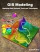
For
example, a pipeline is frequently divided into “stationing coordinates” that
partitions a serpentine route into uniform linear distances along a pipeline (Uniform segmentation). Alternatively, the route can be segmented by
identifying a point at each major change in direction as shown in the top right
portion of figure 1. The result divides
the route into a set of variable length segments responding to planimetric
orientation of straight line sections (Deflection
Angle segmentation).
A more
complex form of segmentation is often referred to as “dynamic segmentation.” This approach uses changes in conditions on
other map layers to subdivide a route.
The Conditions-based
segmentation procedure first derives a “universal conditions” map by overlaying
a set of map layers to establish individual coincident polygons containing the
same combination of conditions throughout their interiors (left side of figure
1). A route is intersected with the
universal conditions map and “broken” into a series of line segments at the
entry and exit of each universal condition polygon.
Figure
1. Basic approaches used in route segmentation.
The result
is a series of variable length line segments with uniform conditions throughout
their length. The line segment set is
written to a table containing x, y and z coordinates followed by fields
identifying the combination of conditions along each segment. In addition, the table can report “crossing
counts” that note the number of intersections of the derived line segments and
other linear features, such as river and road crossings.
Another
advanced form of segmentation involves breaking a route into segments
considering elevation changes along a terrain surface as shown in the bottom
right portion of figure 1. Terrain-based segmentation
divides the route into segments representing similar terrain configuration as
determined by major inflection points and slope conditions.
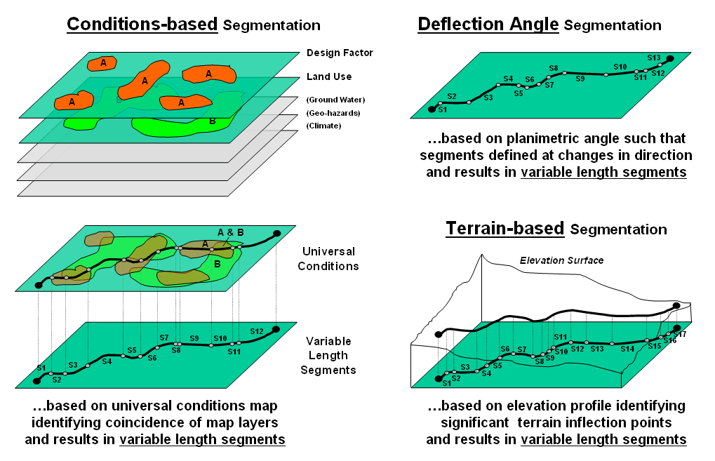
The
first step is to establish the elevation profile of the route by “masking” the
terrain surface with the route. To
eliminate subtle changes, the elevation values are smoothed to characterize the
overall trend of the terrain. This is
done by passing a moving-average window along the elevation profile resulting
in a smoothed profile.
The
width of the smoothing window is critical because if it is too large the
smoothing will eliminate potentially important inflection points; if it is too
small there will be a multitude of insignificant segment breaks. The dilemma is similar to choosing an
appropriate angular change factor in Deflection-angle segmentation and is as
much art as it is science. Experience
for liquid pipelines suggests an 11 to 15-cell diameter window on a 10 meter
digital elevation model (DEM) works fairly well.
Figure
2. Analyzing the slope differences along a proposed route.
Figure
2 illustrates the final step in the procedure.
The tool evaluates the smoothed elevation values by subtracting the
current value from the previous location’s value as the solution progresses
left-to-right along the smoothed profile.
If the sign is the same, a continuous “running slope” is indicated. A negative difference indicates an upward
incline; a negative difference indicates a downward descent; zero difference
indicates no change (flat portion). A
location where the sign of the difference changes (negative to positive;
positive to negative) identifies an inflection point. The coordinates and elevation value for the
location that changed sign is written to a Segments Table.
For
example, the calculations in the upper left portion of figure 2 show a
continued upward incline until the elevation point of 124 is encountered. At this location the sign of the difference
changes indicating the start of a downward descent (from a negative to a
positive difference).
A
refinement to the approach avoids storing and processing the entire elevation
profile of actual values by calculating and comparing the moving average values
(smoothed elevation) on-the-fly. This
approach is much more efficient and greatly improves performance. In this application a 1x15 cell window is
used to smooth the actual elevation profile and store the information in a
temporary table with just two records—previous and current average.
The
difference is calculated and tested for a change in sign; if different, the
coordinates and elevation value for the current location is written to the
Segments Table. The window is advanced
and the old previous average is replaced and a new smoothed value for the current
location is considered. The sequence of
steps of 1) replace, 2) calculate, 3) compare and 4) write if sign change is
repeated until the entire profile of a route has been evaluated.
The
result is a set of map segments with consistent terrain configuration. Summarizing the average slope along the
segmented file provides important information for assessing the hydraulics
along a pipeline and pump-station positioning and design required for
anticipated product flows …a big step beyond simply mapping a pipeline route.
The Long
and Short of Slope
(GeoWorld, July 2007)
Recall
from the past sections dealing with slope calculation that the nine elevation
values in a 3x3 window are generally used.
There are two basic approaches for characterizing relative
steepness—surface fitting and individual slope statistics.
Surface
fitting aligns a plane to the elevation values that minimizes the deviations
from the plane to the values. If all of
the values are the same, a horizontal plane is fitted and the slope is
zero. However as the values on one side
of the window increase and the values on the other decrease, the fitted plane
tilts indicating increasing terrain steepness.
The surface
fitting algorithm first establishes the 3x3 window, then identifies the nine
elevation values, fits the plane and records the slope for the center cell in
the window. The “roving window” shifts
to the next adjacent location and repeats the process until all of the cells in
a project area have been evaluated.
The
algorithm for summarizing individual slopes also utilizes a 3x3 window, but
instead of fitting a plane it calculates the slopes formed by the center
location and each of
its eight neighbors. The
minimum, maximum or average of the individual slope values is recorded for the
center cell and the window advanced.
Both
slope techniques result in a continuous map surface indicating the relative
steepness throughout a project area.
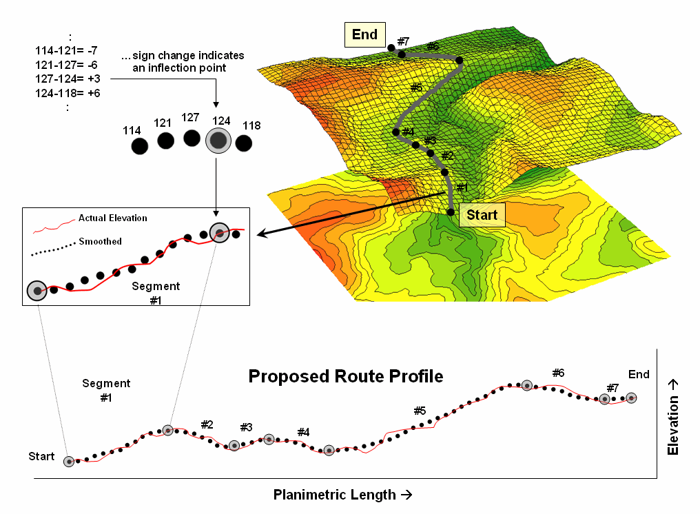
Sometimes, however, slope along a linear feature, such as a pipeline, is
sought (figure 1). In this case, only three cells are involved—the center cell
and its input and output neighbors at each location along the pipeline.
Figure
1. Longitudinal slope calculates the steepness
along a linear feature, such as a pipeline.
Longitudinal Slope (LS)
requires isolating just the route’s elevation values. In grid-based modeling this means first
creating a “masking map” of the route where the cells defining the pipeline are
assigned the value 1 and the non-pipeline cells are assigned a special value of
Null (or No Data). This map is
multiplied by the elevation surface having the effect of retaining the
elevation values along the route but all other locations are assigned Null.
Most
map analysis packages have been “trained” to recognize a Null value and simply
skip over these locations when processing.
The effect in this case is to calculate slope using just the three
aligned elevation values in the 3x3 roving window—either fitted or
maximum/minimum/average.
A
simple extension to the algorithm, Directional
Slope (DS), enables a user to enter a starting location and the direction
of flow, and then it calculates individual slopes for each step along the route
using just the input and center cell.
This technique characterizes where gravity is helping or hindering flow
and is useful in determining draw-down if the pipe is ruptured.
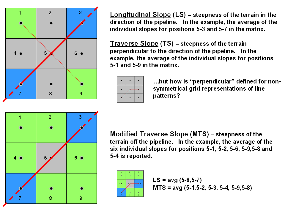
Figure
2. Modified transverse slope is calculated as the
average of off-route slopes surrounding a location.
A more
radical extension considers the off-route cells in calculating Transverse Slope (TS). Traditionally, transverse slope was manually
calculated by estimating the slope of a line perpendicular to the route. For example in the upper portion of figure 2,
the slopes from the center cell (5) to the NE (5-3) and SW (5-7) cells identify
the longitudinal slope along the route while the slopes to the NW (5-11) and SE
(5-9) cells indicate the transverse slope.
The
perpendicular approach works for any orthogonal and diagonal transect of the
window. The elevation grid, however, can
take an oblique bend involving diagonal and orthogonal directions as shown and
there isn’t a true perpendicular. In
this instance, GIS-derived transverse slope requires a new definition.
Modified Transverse Slope (MTS)
calculates slope for the off-route cells, regardless of the linear shape. In the lower-left portion of figure 2 all of
green cells (1, 2, 4, 6, 8 and 9) are considered in calculating terrain
steepness surrounding the pipeline.
Ideally, routes with fairly gentle modified transverse slopes are
preferred as subsidence risks are lower.
These
fairly innocuous extensions for calculating slope point to a bigger issue in
map analysis—mainly that our grid-based analytical toolbox and GIS modeling
expressions are a long way from complete.
Most of the development occurred in the 1970s and 80s and coding of new
capabilities in flagship systems have languished. As a result, solution providers are encoding
specialized tools for their clients and running them outside the GIS or hooking
them in as objects or add-ins.
What I
find interesting is that this is where GIS was in the 1970s and early 80s—a
collection of disparate proprietary systems.
With all that you hear about data standards, open systems and GIS
community access it’s peculiar that map analysis seems to be moving in the
opposite direction.
Identifying
Upland Ridges
(GeoWorld, May 2009)
The
good news is that there is a tsunami of mapped data out there; the bad news is
that there is a tsunami of mapped data out there. Rarely is it as simple as downloading and
displaying the ideal map for decision-making.
More often than not the base data that is available is just that—a base
for further exploration and translation into meaningful information for solutions
well-beyond a basic wall decoration.
Digital
Elevation Models (DEMs) are no exception.
While there is an ever increasing wealth of elevation data at ever
increasing detail, most applications require a translation of the ups and downs
into decision contexts. For example,
suppose you are interested in identifying upland ridges in mountainous terrain
for wildfire considerations, wind power location or animal corridors. Downloading and displaying a set of DEMs
provides a qualitative glimpse at the topography but most human interpretation
becomes overwhelmed by the sheer magnitude of the possibilities and the
inability to apply a consistent definition.
A
topographic ridge can be defined as a long narrow upper section or raised crest
of elevation formed by the juncture of two sloping planes. While the definition of a ridge is
straightforward, its practical expression is a bit murkier. Figure 1 outlines a commonly used grid-based
map analysis procedure for identifying ridges.
The first step involves “smoothing” the surface to eliminate subtle and
often artificial elevation changes. This
is accomplished by moving a small “roving window” over the surface that
averages the localized elevation values in the vicinity of each map location (1 Scan).
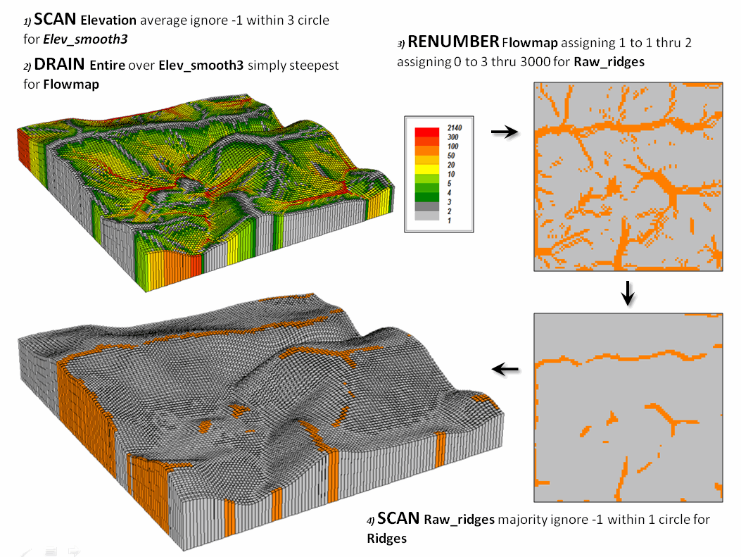
Figure
1. Accumulated surface flow is used to identify
candidate ridges.
(MapCalcTM
software commands are indicated to illustrate processing options)
The
next step simulates water falling across the entire project area and moving
downhill by the steepest path (2 Drain). The computer keeps track of how many uphill
locations contribute water to each grid location to generate the flow
accumulation map draped over the smoothed elevation surface shown in the
upper-left portion of the figure. Note
that lower values (grey tones) indicate locations with minimal uphill
contributors and align with the elevation crests.
The
third step reclassifies the flow map to isolate the locations containing just
one runoff path—candidate ridges (3
Renumber). However note the
cluttered pattern of the map in the upper-right that confuses a consistent and
practical definition of a ridge. The
final step in the figure uses another roving window operation to assign the
majority value in the vicinity of each map location thereby eliminating the
“salt and pepper” pattern of the raw ridges (4 Scan). If most of the
values in the window are 0 (not a potential ridge) then the location is
assigned 0. However if there is a
majority of potential ridges in the window then a 1 is assigned. The draped display in the lower-left confirms
the alignment of the derived ridges with the terrain surface.
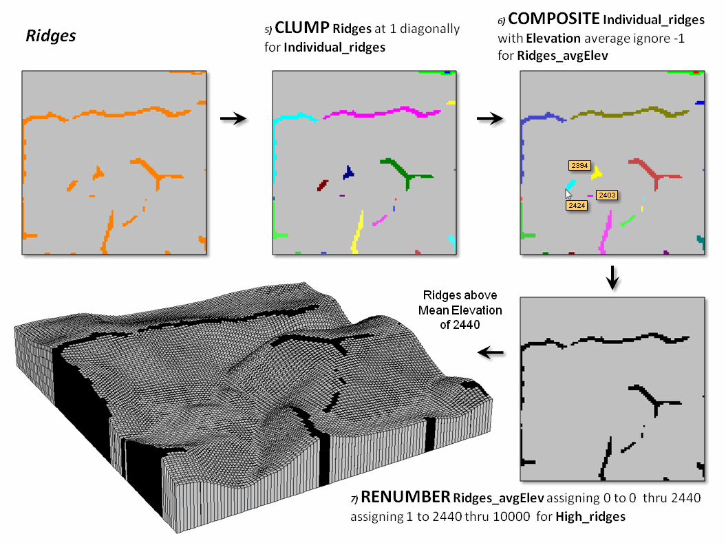
Figure
2. Low ridges are identified and eliminated.
Figure
2 continues the processing to identify just the upland ridges. Contiguous ridge locations are individually
identified (5 Clump) and then the average
elevation for each ridge grouping is determined (6 Composite). Note the low
average elevation of the three small ridges in the center portion of the
project area. The final step in the
figure (7 Renumber) eliminates
candidate ridges that are below the average elevation of the project area
thereby leaving only the high ridge locations (black).
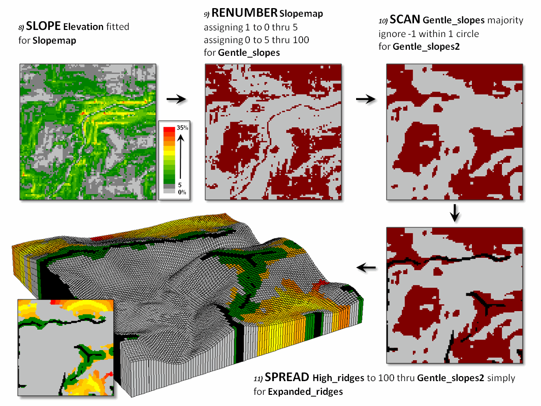
Figure
3. The ridges are extended into surrounding
gently sloped areas to identify effective upland ridges.
Figure
3 illustrates the processing steps for expanding the ridges as a function of
terrain steepness. A slope map is
generated (8 Slope) and calibrated to
isolate areas of gentle slopes of 0 to 5 percent (9 Renumber). In turn, these
areas are processed to eliminate the “salt and pepper” pattern (10 Scan) leaving relatively large
expanses of gentle slopes.
The lower-right map identifies the upland ridges (black)
superimposed on the gently sloped areas (red).
An effective distance operation (11
Spread) is used to extend the ridges considering the non-gently sloped
locations (grey) as absolute barriers.
The warmer tones in the proximity map draped on the elevation surface
indicate increasing distance from a ridge into the surrounding relatively flat
areas. Depending on the application the
upland ridge expansion could be reclassified from the full extent to just the immediate
surrounding areas (green).
The simple model may be extended to characterize
conditions within the derived ridges.
For example, an aspect map can be combined with the extended ridges to
indicate their overall terrain orientation or precise azimuth each grid
location defining the upland ridges to consider for prevailing wind direction
or solar exposure. Another extension
could generate an overland travel-time or a road construction surface to
consider relative access potential of the ridges.
The bottom line is that it takes a bit of spatial
reasoning to translate base maps into decision contexts …it’s the analytic
nature of GIS that moves it beyond mapping.
Generating
Mountains and Molehills from Field Sampled Data
(GeoWorld, August 2013)
Geotechnology has
revolutionized the dogma, development and dissemination of spatial
information—duh. Today’s youth is
growing up in an increasingly cyber-based society with instantaneous connection
to the world about them, and like Peter Pan they can be whisked-away by Google
Earth to distant lands in the blink of an eye.
But what if they are
interested in detail beyond the maximum level of the zoom slider bar? Or they want to simulate localized surface
flow paths, convergence and path density?
Or identify subtle hummocks and depressions? Or model subsurface moisture regimes? Or
relate any of these characteristics to the spatial relationships with
vegetative patterns?
That’s
the dilemma of many aspiring scientists who want to go beyond simply
visualizing a landscape to investigating system interactions that are spatially
driven. But their data analysis quiver
is primarily full of non-spatial analytic tools that rely on assessing and
comparing the central tendencies of field collected data without consideration
of the spatial distributions inherent in the data.
Two
major obstacles stand in their way— appropriate spatial data and spatially
aware analysis tools. Most readily downloadable
data is too course for detailed scientific study, and even if it were
available, most potential users are unacquainted with the quantitative analysis
procedures involved.
Let’s
consider the data limitation hurdle first and then see how its practical
solution can spark spatial reasoning among non-GIS’ers. Suppose a budding grad student wants to
develop a micro-terrain surface for a project area. Unless there is a Lidar
over flight or total station survey of the area available, they will need to
construct a detailed elevation surface from scratch.
First
impulse is to use an inexpensive GPS unit (or Google’s GPS Surveyor app for Smartphones) to
capture XYZ measurements throughout a project area. But alas, it is soon discovered that
precision of the coordinates is insufficient for detailed mapping. The vertical precision in a GPS unit is
characteristically less than half of that of the horizontal precision which in
itself is plus or minus several meters—hardly the precision required for surface
modeling.
Another
possibility is to acquire sophisticated surveying equipment (transit, theodolite, laser
rangefinder or GPS total station), but their costs are far too high both in
terms of a tight budget and a demanding learning curve. A Dumpy level, tripod, graduated staff and a
couple of meter tapes form a far more practical option (they are likely buried
in an old storeroom on campus).
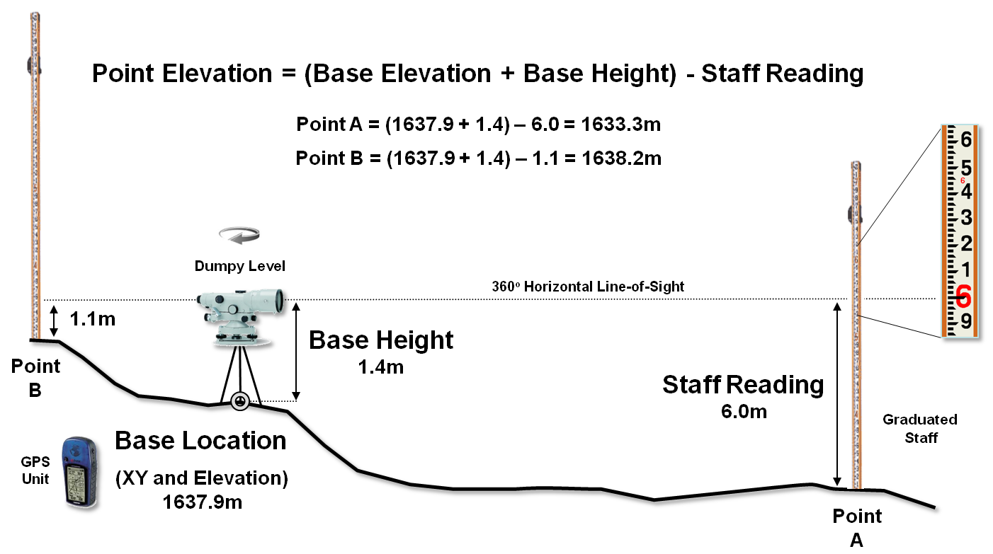
Figure 1. A Dumpy level establishes a horizontal plane to
measure the relative elevation differences throughout a project area.
Dumpy
levels work by precisely measuring vertical distances in a horizontal plane
about a base location (figure 1). A
bubble level is used to establish a horizontal plane in each quarter-circle to
make sure it is level throughout the entire 360 degree swing of the
instrument. An operator looks through
the eyepiece of the telescope, while an assistant slowly rocks a graduated
staff at a sample location and the maximum reading on the staff is
recorded. Subtracting the Staff Reading
from the Base Height determines the relative elevation of any measured point to
a fraction of centimeter.
To
establish real-world positioning, an inexpensive GPS unit can be used. The average of several readings taken
throughout the day provides a “reasonable estimate” of the Base Location’s
earth position (top-right portion of figure 2).
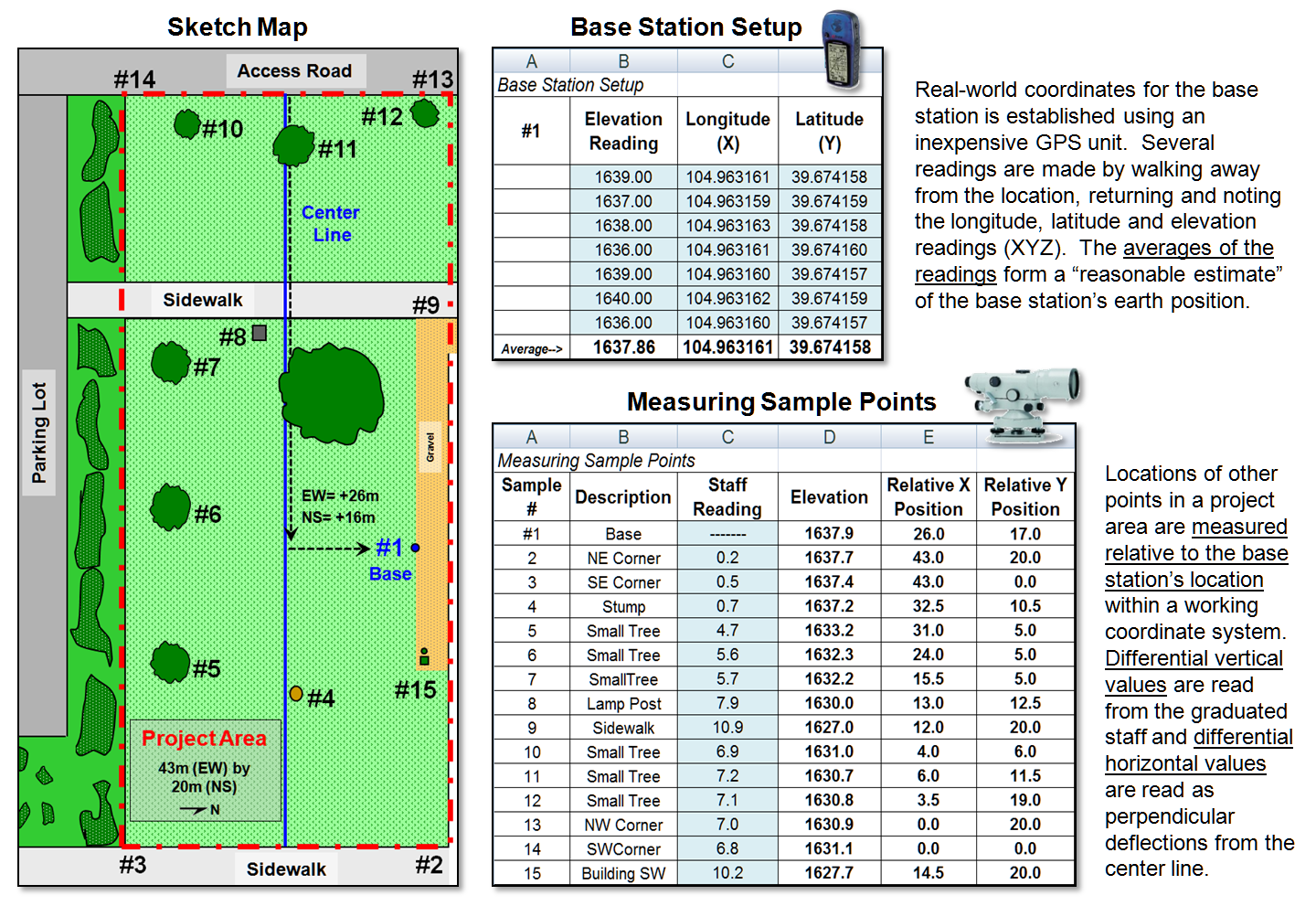
Figure 2. The XYZ coordinates of sample points are easily
derived from field data.
Before
the staff is moved to another location, the distance along a center line is measured
(EW as the X axis in the example) and the perpendicular deflection to the point
is measured (NS as the Y axis). The
result is a record of relative horizontal location and elevation difference
that is easily evaluated for XYZ coordinates within a working coordinate system
(bottom-right portion of figure 2) or relative to the base station’s Lat/Lon
real-world coordinates.
The final step involves
surface modeling software to complete the 3-dimentional surface by “spatially
interpolating” the elevation values for all of the grid cells within the
project area. Figure 3 shows the result
using the powerful yet inexpensive Surfer software package (by Golden
Software). The derived terrain surface
can be exported to ArcGIS, MapCalc or other map analysis package, as well as to
Google Earth as contour lines or a color-shaded raster image.
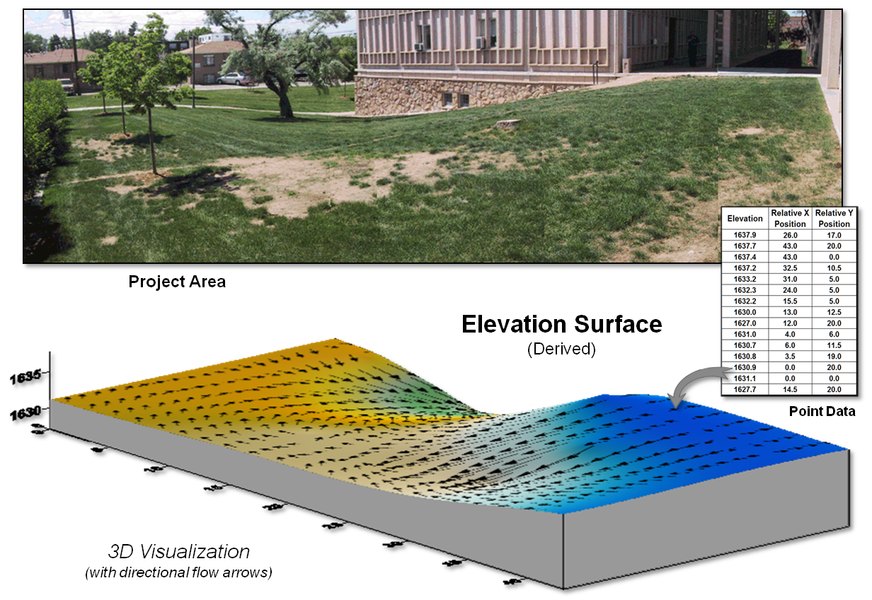
Figure 3. A detailed elevation surface is generated using
inexpensive surface modeling software.
I have presented this
3-hour workshop in various forms to numerous GIS and non-GIS students and
professionals since the 1980s. The
practical fieldwork coupled with easy-to-use software encourages dialog about
the inherent spatial nature ingrained in most field collected data.
Discussion quickly
extends to data other than elevation—the “Z values” could easily be relative
concentrations of an environmental variable; or disease occurrences in an
epidemiological study; or relative biomass or stem density measurements of a
plant species; or crime incidences for mapping pockets of crime in a city; or
point of sales values for a particular product; or questionnaire response levels
in a social survey; etc.
The peaks and valleys in
any map surface characterize the spatial distribution of that mapped variable—
identifying where the relative highs and lows occur in geographic space. And since a map surface is a spatially organized
set of numbers, mathematical and statistical analysis tools can be
applied.
The bottom line is that
many (most?) field-based mapped data contain useful information about the
spatial distribution/pattern inherent in the data. While the ability to surface map this
characteristic is well-known within the GIS community, it is less familiar and
woefully underutilized in the applied sciences.
A simple experience in surface mapping terrain elevation can be useful in
crossing this conceptual chasm and often serves as a Rosetta stone in
stimulating cross-discipline discussion and recognition of “maps as data”
awaiting quantitative analysis— as opposed to traditional “graphic images” for
human viewing and interpretation.
Altering
Our Spatial Perspective through Dynamic Windows
(GeoWorld, August 2012)
The use of “roving
windows” to summarize terrain configuration is well established. The position and relative
magnitude of surrounding values at a location on an elevation surface have long
been used to calculate localized terrain steepness/slope and
orientation/aspect.
A
search radius and geometric shape of the window are specified, then surface
values within the window are retrieved, a summary technique applied (e.g.,
slope, aspect, average, coefficient of variation, etc.) and the resulting
summary value assigned to the center cell.
The roving window is systematically moved throughout the surface to
create a map of the desired surface summary.
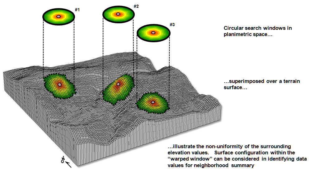
Figure 1. Fixed windows form circles in planimetric space but
become warped when fitted to a three-dimensional surface.
The top
portion of figure 1 illustrates the planimetric configuration of three
locations of a circular fixed window with a radius of ten
grid spaces. When superimposed onto the
surface, the shape is warped to conform to the relative elevation values
occurring within the window. Note that
the first location is moderately sloped toward the south; second location is
steeply sloped toward the west; and the third location is fairly flat with no
discernible orientation.
What you
eye detects is easily summarized by mathematical algorithms with the resultant
values for all of the surface locations creating continuous maps of landform
character, such as surface roughness, tilted area and convexity/concavity, as
well as slope and aspect.
A weighted
window is a variant on the simple fixed window that involves
preferential weighting of nearby data values.
For example, inverse distance weighted interpolation uses a fixed
shape/size of a roving window to identify data samples that are weight-averaged
to favor nearer sample values more than distant ones. Or a user-specified weighting kernel can be
specified as a decay function or any other weighting preference, such as
assigning more importance to easterly conditions to account for strong and dry
Santa Ana winds when modeling wildfire threat in southern California. It is common sense that these easterly
conditions are more influential than just a simple or distance-weighted average
in all directions.
Dynamic
windows
use the same basic processing flow but do not use a fixed reach or consistent
geometric shape in defining a roving window.
Rather, the size and shape is dependent on the conditions at each map
location and varies as the window is moved over a map surface.
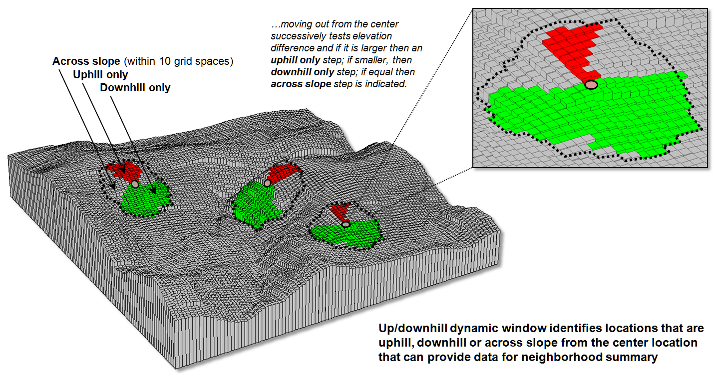
Figure 2. Uphill, downhill and across portions of a roving
window can be determined by considering the relative values on a
three-dimensional surface.
For
example, figure 2 depicts a roving window based on uphill, downhill and across
slope movements from the center location.
Lots of spatial processes respond differently to these basic landform
conditions. For example, uphill
conditions can contribute surface runoff to the center cell, downhill locations
can receive flows from the center cell and sediment movement at the across
slope locations is independent of the center cell. Wildfire movement, on the
other hand, is most rapid uphill, particularly in steep terrain, due to
preheating of forest fuels. Hence,
downhill conditions are more important in modeling threat at a location than
either the across or uphill surrounding conditions.
Another
dynamic consideration is effective distance.
For example, a window’s geographic reach and direction can be a function
of intervening conditions, such as the relative habitat preference when
considering the surroundings in a wildlife model. The window will expand and contract depending
on neighboring conditions forming an ameba-like shape to identify data values
to be summarized—the pseudopods change shape and extent at each instantaneous
location. The result is a localized
summary of data, such as proximity to human activity within preferential reach
of each grid location to characterize animal/human interaction potential.
Or a
combination of window considerations can be applied, such as (1) preferential
weighting of the fuel loadings (2) along downhill locations (3) as a function
of slope with steep areas reaching farther away than gently sloped areas. In a wildfire risk model, the resultant
“roving window” summary would favor the fuel conditions within the elongated
pseudopods of the steeply sloped downhill locations.
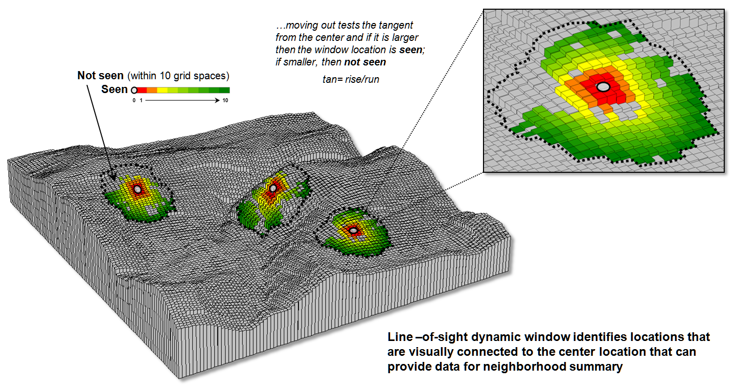
Figure 3. A line-of-sight window identifies locations that
are seen and not seen from the window’s focus.
A third
type of dynamic consideration involves line-of-sight connectivity where the
“viewshed” of a location within a specified distance is used to define a roving
window (see figure 3). In a military
situation, this type of window might be useful in summarizing the likelihood of
enemy activity that is visually connected to each map location. Areas with high visual exposure levels being
poor places to setup camp, but ideal
places for establishing forward observer outposts.
A less
war-like application of line-of-sight windows involves terrain analysis. Areas not seen are “over the hill” in a macro-sense
for ridge lines and “in a slight depression” in a micro-sense for
potholes. If all locations are seen then
there is minimal macro or micro terrain variations.
The rub
is that most of the user community and much of the vector-based GIS’ers are unaware
of even fixed roving windows, much less weighted and dynamic windows. However, the utility of these advanced
procedures in conceptualizing geographic space within context of its
surroundings is revolutionary. The view
through a dynamic window is as useful as it is initially mind-boggling …see you
on the other side.
____________________________________________
Further Online Reading: (Chronological
listing posted at www.innovativegis.com/basis/BeyondMappingSeries/)
Shedding
Light on Terrain Analysis — discusses how terrain orientation is
used to generate Hillshade maps (May 2008)
(Back
to the Table of Contents)