|
Beyond
Mapping IV Topic 3
– Extending Terrain Analysis Procedures (Further Reading) |
GIS Modeling book |
Shedding
Light on Terrain Analysis — discusses how terrain
orientation is used to generate Hillshade maps (May 2008)
<Click here> for a printer-friendly version of this topic (.pdf).
(Back
to the Table of Contents)
______________________________
Shedding Light on Terrain Analysis
(GeoWorld, may
2008)
A lot of GIS is straightforward and mimics our boy/girl scout days
wrestling with paper maps. We learned
that North is at the top (at least for us in the northern latitudes) and red
roads and blue streams wind their way around green globs of forested
areas. However, the brown concentric
rings presented a bit more of a conceptual challenge.
When the contour lines formed a fairly small circle it was likely a
hilltop; or a depression, if the line sprouted whiskers. Sharp “V-shaped” contour lines pointed
upstream when a blue line was present; and somewhat rounded V’s pointed
downhill along a ridge. Once these and a
few other subtle nuances were mastered and you survived a day or so in the woods,
a merit badge and sense power over geography was attained.
Your computer is devoid of such a nostalgic experience. All it sees are organized sets of colorless
numbers. In the case of vector systems,
these number sets identify lines defining discrete spatial features in a manner
fairly analogous to traditional mapping.
On the surface, direction measurement fundamentals remain the same and
your fond memory of the 0-360o markings around a compass ring holds
for most GIS mapping applications.
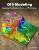
The upper-left portion of figure 1 unfolds the compass ring into a
continuum of azimuth from 0o (north) to 360o
(north). Whoa …you mean north is at both
ends of the continuum? As azimuth
increases, it becomes less north-like for awhile and then more north-like until
0 = 360. Now that’s enough to really
mess-up a numeric bean-counter like a computer.
Actually, azimuthal direction is termed a discontinuous number set as it
wraps around on itself (spiral in the top-right side of figure 1).
The lower scales in figure 1 transform direction into a more stable
continuous number set that indicates the relative alignment with a specified
direction. A Facing Angle
utilizes the concept of a back azimuth to indicate an orientation as different
as it gets—180o is completely opposite; and 0o is exactly
the same direction.
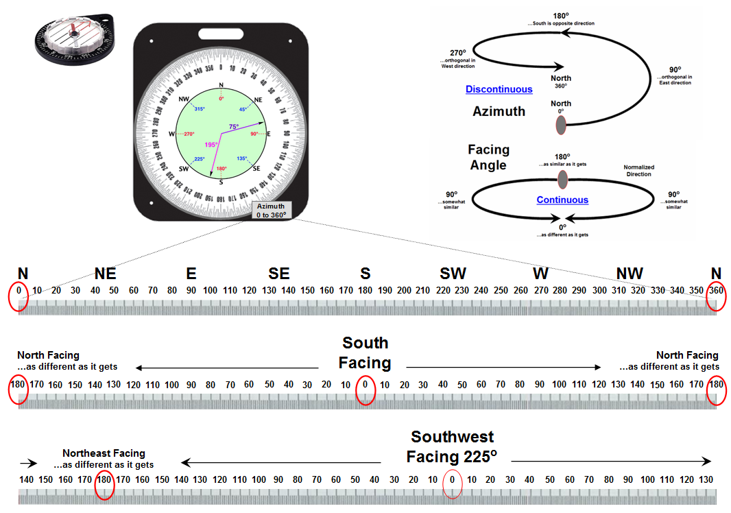
Figure 1. Azimuth is a discontinuous numeric scale as
it wraps around on itself; Facing Angle is a continuous gradient indicating
relative alignment with a specified direction.
For a south facing location the continuum starts at 0 (South) and
progresses “less south-like” in both the East and West directions until the
orientation “is 180 degrees off” at due North.
The importance of the consistency of this continuous scale might be lost
on humans, but it means the world to a computer attempting to statistically
analyze a set of directional data. The
procedure normalizes terrain data for any given facing angle into a consistent
scale of 0 to 180 indicating the degree of orientation similarly throughout an
entire project area.
Figure 2 summarizes the geometry between Azimuth and Facing
angles. Also it introduces the concept
of a Horizontal angle that takes direction from 2D planar to 3D solid
geometry. The “Hillshade” map of
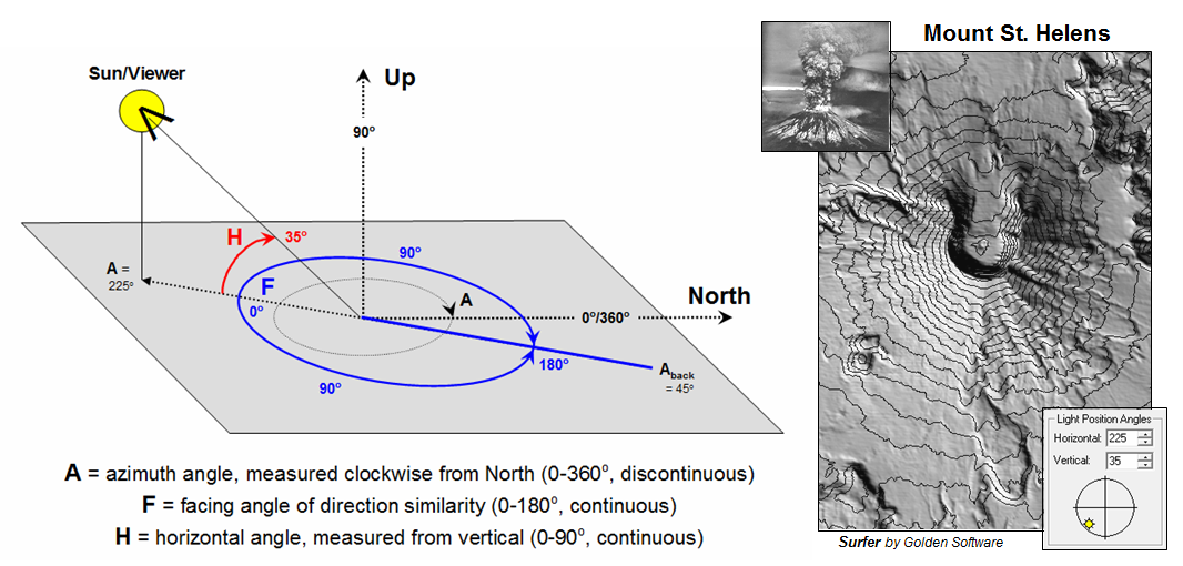
Figure 2. A Hillshade map identifies the relative
brightness at every grid location in a project area.
Figure 3. Terrain orientation combines azimuthal and
horizontal angles for each grid cell facet.
Figure 3 expresses the relationship between the azimuth and horizontal
angle gradients derived from aspect and slope maps. Each grid cell (30x30 meters in this example)
can be thought of as a tilted plane in three-dimensional space. In the case of the brightest location, it
identifies a grid cell that is perpendicular to the sun—like a contented lizard
or sunbather positioned to absorb the most rays. All other possible orientations of the grid
cell facets are some combination of the facing and horizontal angle gradients.
However, the “superstar map-ematicians” among us know that things
are a bit more complex than an independent peek at each grid cell. A grid cell could be directly oriented toward
the sun but on a small hill in the shadow of a much larger hill. To account for the surrounding terrain
configuration one needs to solve the angles using solid geometry algorithms
involving direction cosines to connect the grid cell to the sun and test if
there is any intervening terrain blocking connection.
So what’s the take-home from all this discussion? Actually three points should stand out. First, that GIS technology encompasses our
paper map thinking (e.g., discontinuous azimuthal direction), but the digital
map enables us to go beyond mapping.
Secondly, that a map is an organized set of numbers first, and a picture
later; we must understand the nature of the data (e.g., continuous facing
angle) to fully capitalize on the potential of map analysis.
Finally, the new map-ematical expression of maps supports
radically new applications. For example,
one can integrate a series of brightness maps over a day for a map of solar
influx (insolation) that drives a wealth of spatial systems from wildlife
habitat to global warming. In addition,
these data can be statistically analyzed for insight into spatial patterns,
relationships and dependencies that were beyond discovery a few years ago. In short, GIS is ushering in a new era of
decision-making, not simply keeping track of where is what.
_____________________________
Author’s
Note: related discussion on Terrain Analysis is in Topic 6, Summarizing
Neighbors in the book Map Analysis (Berry, 2007; GeoTec Media, www.geoplace.com/books/MapAnalysis)
and Topic 11 in the online Beyond Mapping
Correction: the following letter
(5/25/08) outlined some concerns about the discussion of Azimuth.
Joseph— in the many years of Beyond Mapping I’ve never had a serious
disagreement. In the May column it seems
as though your slant on angles is a bit off course. I’m no map-ematician but azimuth is not
discontinuous; rather it is a cyclic attribute type that continuously wraps
around (and around). If we thought of
phase angles as discontinuous we would have a hard time using sines and cosines
to compute mean wind directions slope aspects or buoy longitudes east of New
Zealand.
You say too that the brightest areas in a hillshade image face the
sun. Those slopes that exactly face the
sun reflect light back to the sun’s incident angle, not the viewer. When the angle of incidence from surfaces is
oblique to the sun angle it causes the angle of reflection to return to the
viewer “overhead” the surface is brightest.
One more thing if you will allow me.
Your Mount St. Helens is lit from 225 degrees, putting the
“shadows” to the north-east. This
violates the remote sensing custom of putting the “shadows” to the south-east
to avoid the terrain inversion phenomenon that results from the pseudoscopic
effect. Many folks will see your Mt. St.
Helens, as a depression with a small Mound St. Helens at the bottom. That of course is why the Surfer default is
335 degrees.
Best wishes, Peter H. Dana, Ph.D., Research Fellow and Lecturer,
Department of Geography, University of Texas at Austin, pdana@mail.utexas.edu
Peter— right on … excellent points well taken. Azimuth is not
“discontinuous” and your classification of “cyclical” is a good one. The
bottom line is that azimuth isn’t your normal numerical gradient and being a
bit whacko one can’t simply utilize raw azimuth values in spatial data
mining.
My use of the term “brightest areas” was misleading …I was referring to
surface illumination intensity (amount of sunlight impacting a location as
contained in the facing angle) not the relative brightness in the image which
is dependent on viewer angle as well as solar angle as compounded by the unique
lay of the terrain.
Your recounting of the imaging interpretation rule also holds true for
interpreting the graphic. My point however was less on the interpretation
of the map graphic as on the ability to track solar insolation …mapped data
versus visualization. The bottom line is that I am delighted that someone
out there actually reads the column, particularly with your level of interest
and expertise. The dialog is much appreciated and I stand
corrected. Thank you. Joe
(Back to the Table of Contents)