|
The Precision Farming Primer |
|
|
|

Overview
of the Case Study
”Some Assembly” Required in Precision Ag
Mapped Data Visualization and Summary
Preprocessing and Map Normalization
Exchanging Mapped Data
Comparing Yield Maps
Comparing Yield Surfaces
From Point Data to Map Surfaces
Benchmarking Interpolation Results
Assessing Interpolation Performance
Calculating Similarity Within A Field
Identifying Data Zones
Mapping Data Clusters
Predicting Maps
Stratifying Maps for Better Predictions
Spatial Analysis Operations
(return to Table
of Contents)
Overview of the Case Study (return to top)
 Author’s note: An educational version of the MapCalc
software by Red Hen Systems used in the case study provides “hands-on”
exercises for the topics discussed in this appendix. See www.redhensystems.com for more
information and ordering; US$21.95 for Student CD and US$495.00 for Instructor
CD with multi-seat license for a computer lab (prices subject to change).
Author’s note: An educational version of the MapCalc
software by Red Hen Systems used in the case study provides “hands-on”
exercises for the topics discussed in this appendix. See www.redhensystems.com for more
information and ordering; US$21.95 for Student CD and US$495.00 for Instructor
CD with multi-seat license for a computer lab (prices subject to change).
Now
that precision farming is beginning its second decade, where are we? Yield mapping is gaining commonplace status
for many crops and locales. Site-specific
management of field fertilization has a growing number of users. Remote sensing applications from satellite
imagery to aerial photos and on the ground “proximal” sensing are coming
onboard. Irrigation control, field
leveling, variable rate seeding, on-farm studies, disease/pest modeling, stress
maps and a myriad other computer mapping uses are on the horizon.
Fundamental
to all of these applications are the digital nature of a computer map and the
procedures required to turn these data into useful information for
decision-making. The bottom line for
precision farming appears to be an understanding of the numbers and what one
can do with them to enhance their interpretation.
The
next several columns will apply map analysis techniques in a case study
format. We will begin with a series of
techniques used to visualize and summarize field data and end with several
techniques that develop maps to guide management action. The focus will be on methodology (a.k.a., the
precision farming “toolkit”) and not on the scientific results or
generalizations about the complex biological, adaphic or physiographic factors
driving crop production in the example field.
These intricate relationships are left to agricultural scientists to
scrutinize, interpret and put into context with numerous other crops and
fields.
The
objective of the series of articles simply is to demonstrate the analysis
procedures on a consistent data set. The
intent is to build a case study for a single field that illustrates the wealth
of emerging analysis capabilities that are available to scientists,
agronomists, crop consultants and producers.
One
might argue that we have “the technical cart in front of the scientific
horse.” In many instances that appears
true. We can collect data, view the
numbers as maps or summary statistics, but struggle to make sense of it
all. In part, the disconnect isn’t
technical versus science but the predicament of “the chicken or the egg coming
first.”
We
have a radically different set of analysis tools than those available just ten
years ago. Concurrently, we have a
growing number of farmers collecting geo-registered data, such as crop yield,
soil nutrients and meteorological conditions.
The computer industry is turning out software and machines that are
increasing more powerful, yet costing less and less and are easier to use. The ag equipment companies are developing
implements and instruments that respond to “on the go” movements throughout a
field. In short, the pieces are coming
together.
The
accompanying table lists the topics that will be covered in the series. Most of details of the topics have been
discussed in previous “GIS Toolbox” articles.
What awaits is the demonstration of their application to a consistent
data set. Hopefully, the case study will
stimulate innovative thinking as much as it outlines how the procedures can be
applied. All of the processing will be
done with readily available software for a PC environment.
The
next decade in precision farming will focus on making sense of the
site-specific relationships we measure.
The technology is here (analysis toolbox) to bridge the gap between maps
and decisions. Its widespread
application will be determined by how effective we are in applying it.
Case Study in Agricultural Map Analysis
|
Mapped Data Visualization and Summary |
|
Preprocessing
and Map Normalization |
|
Comparing
Maps and Temporal Analysis |
|
Interpolating
and Assessing Map Surfaces |
|
Integrating
Remote Sensing Data |
|
Delineating
Management Zones |
|
Clustering
Groups of Similar Data |
|
Measuring
Correlation Among Maps |
|
Developing
Predictive Models |
|
Generating
Management Action Maps |
“Some Assembly Required” in Precision Ag (return to top)
Before
we start wrestling with the details of spatial data analysis it makes sense to
consider some larger issues surrounding their application—namely, the interaction
between technology and science, the relevant expression of results,
and the current field-centric orientation of analysis.
The underlying concept of
precision agriculture is that site-specific actions are better than whole-field
ones. In applying fertilizer, for
example, changing the rate and mixture of the nutrients throughout a field puts
more than the average where it is needed and less where it is not needed. However, precise science in the formulation
of prescription maps is critical.
To
date the infusion of site-specific science has not kept pace with the
technologies underlying site-specific agriculture. We can produce maps of yield variation and a
host of potential driving factors, from soil properties and nutrients to
electric conductivity and topographic relief.
We can generate prescription maps that guide the precise application of
various materials. Where we used to use
one recommendation, we now have several for different locations in a
field. So what’s the problem?
It’s
not that there is a problem; it’s just that there is far more potential. Introduction of spatial technology has
forever altered agriculture—for the researcher, as well as the farmer. The traditional research paradigm involves
sampling a very small portion of a field then analyzing these data without reference
to their spatial context and relationships.
The most frequently used method develops a “regression model” of one
variable on another(s), then extrapolates the results for large geographic
regions.
A
classic example is a production curve that relates various levels of a nutrient
to yield—e.g., the Yield vs. Phosphorous plots you encountered in agronomy
101. The interpretation of the curve is
that if a certain level of phosphorous is present, then a certain amount of
yield is expected. This science, plus a
whole lot of field experience (windage), is what goes into a
prescription—whole-field and site-specific alike. If a map of current phosphorous levels
exists, then the application rate can be adjusted so that each location
receives just the right amount to put it at the right spot on the production
curve.
Current
precision ag technology enables just that…site-specific application, but
based on state-wide equations (science). In fact, the “rules” used in most systems
were developed years ago at experiment stations miles away, indifferent to
geographic patterns of topographic, adaphic and biological conditions, and
analyzed with non-spatial statistics that intentionally ignore spatial
autocorrelation.
Today,
an opportunity exists for site-specific science to “tailor” the decision rules
for different conditions within a field.
For example, more phosphorous might be applied to south-facing toe
slopes than north-facing head-slopes.
But the least amount would be applied in flat or depressed areas. Of course the spatially-specific rule set
would change for different soil types and in accordance with the level of
organic matter.
The
primary difference between “non-spatial science” and its spatial cousin is the
analysis of map variables versus a small set of sample plots attempting to replicate
all possible conditions and their extent within a field. Until recent developments there wasn’t a
choice, as the enabling spatial technologies didn’t exist ten years ago.
Now
that we have spatial tools we need to infuse them into agricultural science. Ideally, these activities will gravitate from
the experiment station model to extensive on-farm studies that encompass actual
conditions on a farmer’s land. In
addition, the focus will expand from identifying “management zones” to the
analysis of continuous map surfaces.
Without shifts in perspective, the “whole-field” approach simply will be
replaced by “smaller-field-chunks” (management zones) that blindly apply
non-spatial rule sets. Without fully
engaged science, the full potential of site-specific agriculture will be
aggregated into a series of half steps dictated by technology.
In
addition to a closer science/technology marriage, the results of its
application need to be expressed in new and more informative ways. The introduction of maps has enlightened
farmers and researchers alike to the variability within agricultural
fields. Interactive queries of a stack
of maps identify conditions at specific locations. However, simply presenting base map data
doesn’t always translate into information for decision-making. Further processing is needed to decode these
data into a decision context. For
example, bushels and pounds per acre could be rendered into revenue, cost and
net profit maps under specified market conditions. As the assumptions are changed the economic
maps would change similar to a spreadsheet.
Broadening
the geographic focus of precision agriculture is a third force directing the
future development. To date, most
spatial analysis of farm inputs and outputs stop at the edge of the fields…
like the fields are islands surrounded by nothing. This myopic mindset disregards the larger
geographic context of agriculture.
Increasing environmental concern in farm practices could radically alter
the field focus in the not too distant future.
For
example, the focus might be extended to the surface flows and transport of
materials (fine soil particles, organic matter, chemicals, etc.) that connect a
field to its surroundings. Like forestry
companies, the cumulative environment effects within an air- or watershed might
need to be considered before certain farming activities can take place. The increasing urban/farm interface will
surely alter the need and methods of communication between agriculture and
other parts of society. Spatial analysis
can play a key role in how agricultural stewardship is effectively
communicated.
Precision
agriculture is not going away. The blend
of modern science and technology is like a locomotive with momentum—impossible
to stop. But the direction of the tracks
determines where it goes. Current
decisions by software developers, equipment manufacturers, service providers
and farmers themselves, are laying the groundwork for tomorrow’s direction. Thinking “out of the box” at this stage might
be the best route.
Mapped Data Visualization and Summary (return to top)
The next several columns
will apply map analysis techniques in a case study format. Discussion begins with a series of procedures
used to visualize and summarize field data and ends with several approaches
that develop maps to guide management action.
The map-ematical procedures used to translate data into useful
information is demonstrated using a subset of the data collected for a large
multidisciplinary project of the Water Management Unit of ARS and the
Experiment Station at Colorado State University. The MapCalc software by Red Hen Systems is
used throughout the case study for analysis and display of the data. A set of “hands-on” exercises based on the
case study is available for classroom and self-study (see author’s note).
The most fundamental
concept in analyzing precision farming data is the recognition that all of the
maps are “numbers first, pictures later.” While the human mind is good at a lot of
things, noting subtle differences within large, complex sets of spatial data
isn’t one of them. To visualize these
data we first must aggregate the detailed information into a few discrete
categories then assign colors to each of the groupings.
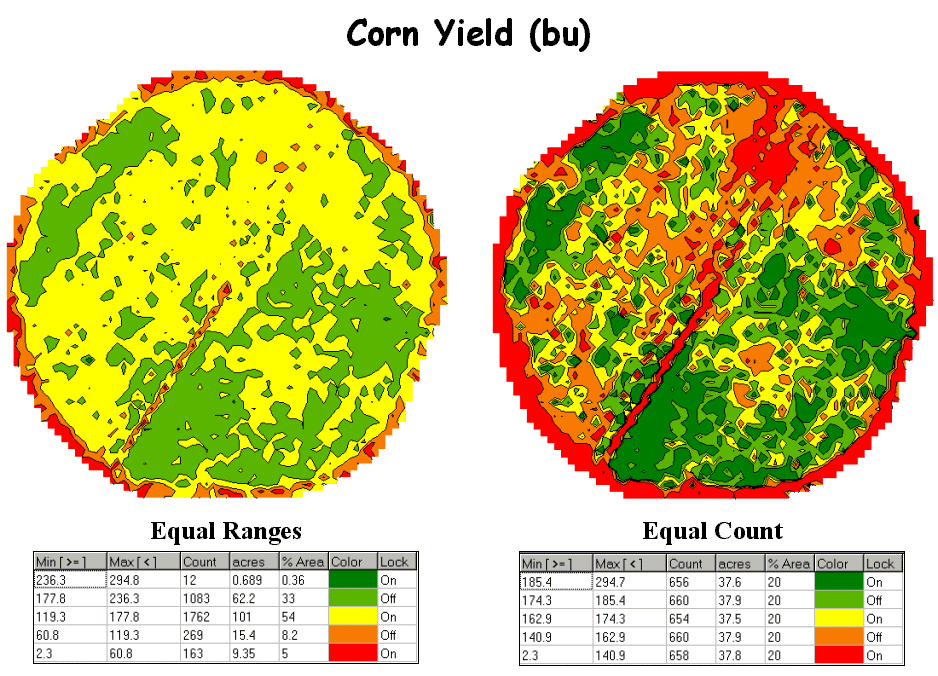 Figure 1. Two
different renderings (categorizations) of yield data.
Figure 1. Two
different renderings (categorizations) of yield data.
For example, the yield maps
shown in figure 1 appear dramatically different but were generated from the
same harvest data. Both maps have five
categories extending from low to high yield and use the same color scheme.
The differences in
appearance arise from the methods used in determining the breakpoints of the
categories—the one on the left uses “Equal Ranges” while the on the right uses
“Equal Count.” Equal Ranges
is similar to
an elevation contour map since it divides the data range (2.33 to 295 bu/ac)
into five steps of about 60 bushels each. Note that the middle interval
(119.3 to 177.8) has more than 100 acres and comprises over half of the field
(54%). Equal Count, on the other hand, divides the same
data into five classes, but this time each category represents about the same
area (20%) and contains a similar number of samples (about 660).
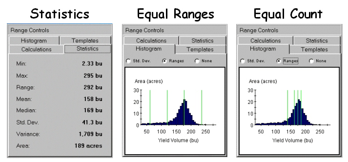 Figure 2.
Statistical summary of yield data.
Figure 2.
Statistical summary of yield data.
The differences between the
two approaches are best visualized from a combined statistical/graphical
perspective. The left panel in figure 2
shows the basic Descriptive Statistics for the data set—min,
max, range, mean, median, standard deviation, variance and total area. While these statistics report a fairly good
harvest overall (an average yield of 158 bu/ac), they fail to map the yield
patterns (spatial variability) throughout the field.
The two histograms on the
right side of figure 2 link the statistical perspective with the map
displays. Recall that a histogram is
simply a plot of the data range (X-axes) versus the number of samples
(Y-axis). The “vertical bars”
superimposed on the histograms identify the breakpoints for the
categories—evenly spaced along the Y-axis for Equal Ranges while variably
spaced for Equal Count. Note the direct
relationship between the placement of the bars and the category intervals shown
in the map legends shown in figure 1.
For example, the first interval begins at 2.3 bushels for both maps but
breaks at 60.8 for Equal Ranges and 140.9 for Equal Count. The differences in the placement of the
breakpoints (vertical bars) account for the differences in the appearance in
the two yield maps.
Similarly, changes in the number
of intervals, and to a lesser degree, changes in the color scheme
will produce different looking maps. By
its very nature, discrete contour mapping aggregates the spatial variability
within field-collected data. The
assignment into categories is inherently a subjective process and any changes
in the contouring parameters result in different map renderings. Since decisions are based on the appearance
of spatial patterns, different actions could be taken depending on which
visualization of the actual data was chosen.
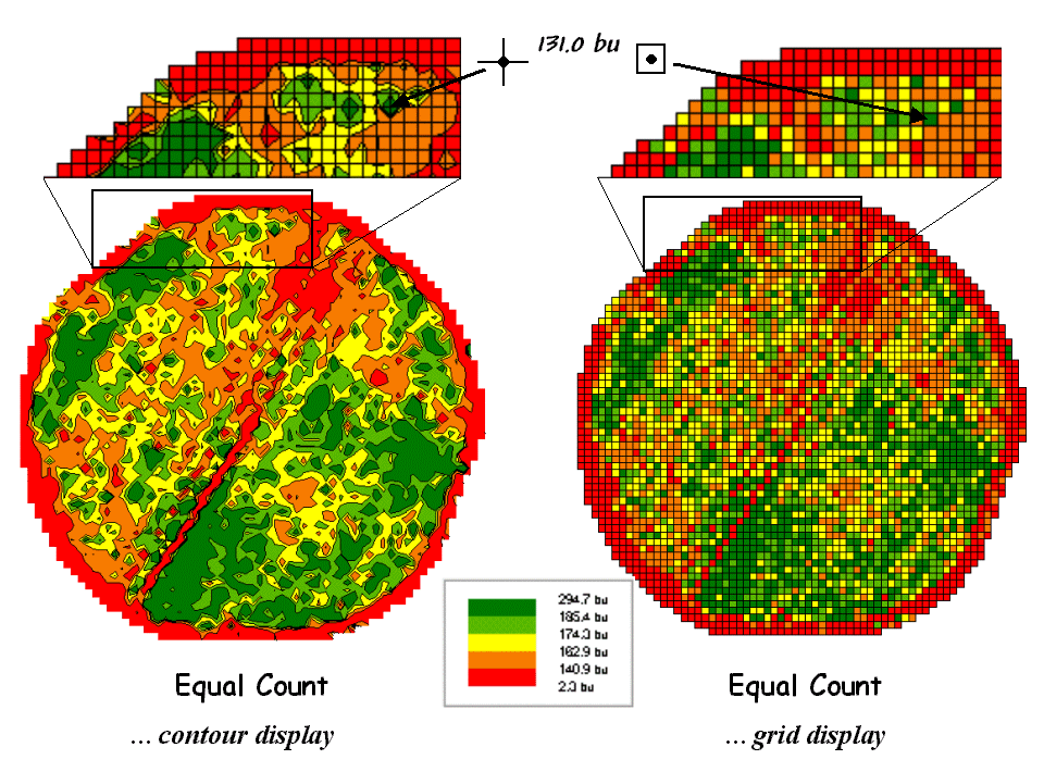 Figure 3. A reference grid is used to directly link the
map display and the stored data.
Figure 3. A reference grid is used to directly link the
map display and the stored data.
The
map on the left-side of figure 3 shows the Equal Count contour map of yield
composed of irregular polygons that identify the discrete categories. The inset directly above the contour map
characterizes the underlying lattice data structure for a portion
of the field. A yield value is stored
for each of the line intersections of the superimposed regular grid. The breakpoint values for the map categories
are plotted along the lines connecting the actual data. The contours are formed by connecting the
breakpoints, smoothing the boundary lines and filling the polygons with the
appropriate color.
The
grid data structure utilizes a superimposed reference grid as
well. However, as depicted in the grid
map and inset on the right side of figure 3, the centroid of each grid cell is
assigned the actual value and the entire cell is filled with the appropriate
color. Note the similarities and
differences in the yield patterns between the contour and grid displays—best
yields generally in the southeast and northwest portions of the field.
Next month’s column will investigate the important considerations in representing precision farming data as continuous map surfaces, viewing these data as 3-D displays and pre-processing procedures used to “normalize” maps for subsequent analysis.
Preprocessing and
Map Normalization (return to top)
Preprocessing and normalization are critical steps in
map analysis that are often overlooked when the sole objective is to generate
graphical output. In analysis, however, map
values and their numerical relationships takes center stage.
Preprocessing involves conversion of raw
data into consistent units that accurately represents field conditions. For example, a yield monitor’s calibration
is used to translate electronic signals into measurements of crop production
units, such as bushels per acre (measure of volume) or tons per hectare
(measure of mass). The appropriate units
(e.g., bushels vs. tons) and measurement system (English acres vs. metric
hectares) is determined and applied to the raw data. While this point is important to software
developers, it is somewhat moot in most practical applications after the
initial installation of software preferences.
A
bit more cantankerous preprocessing concern involves raw data adjustments and
corrections. Like calibrations, adjustments
involve “tweaking” of the values… sort of like a slight turn on that bathroom
scale to alter the reading to what you know is your true weight.
Corrections, on the other hand,
dramatically change measurement values, both numerically and spatially. For example, as discussed in previous columns
the time lag from a combine’s header to the yield monitor can require
considerable repositioning of yield measurements. Also, a combine can pass over the same place
more than once and the duplicate records must be corrected. Even more difficult is the corrections of a
reading from a partial header width or the effects of empting and filling the
thrashing bin as a combine exits from one pass and enters another.
The
old adage “garbage in, garbage out” holds true for any data collection
endeavor. Procedures for calibration,
adjustments and corrections are used to translate raw data measurements into
the most accurate map values possible.
But even the best data often needs a further refinement before it is
ready for analysis.
Normalization involves standardization of
a data set, usually for comparison among different types of data. For example, crop rotation can provide
different views of the productivity of a field.
While direct visual comparison of onion and corn yield maps might
provide insight, some form of normalization of the data is needed prior to any
quantitative analysis. In a sense,
normalization techniques allow you to “compare apples and oranges” using a
standard “mixed fruit scale of numbers.”
The
most basic normalization procedure uses a goal to adjust map
values. For example, a goal of 250
bushels per acre might be used to normalize a yield map for corn. The equation,
Norm_GOAL = (mapValue / 250 ) *
100
derives the percentage of the goal achieved by each
location in a field. In evaluating the
equation, the computer substitutes a map value for a field location, completes
the calculation, stores the result, and then repeats the process for all of the
other map locations.
Insert
B in figure 1 shows the results of goal normalization. Note the differences in the descriptive
statistics between the original and normalized data— a data range of 2.33 to
295 with an average of 158 bushels per acre for the original data versus .934
to 118 with an average of 63.3 percent of the goal.
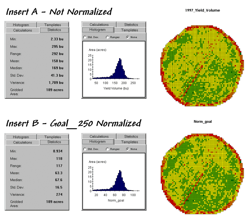 Figure 1. Comparison of original and “goal normalized”
data.
Figure 1. Comparison of original and “goal normalized”
data.
Now note that the two histograms look nearly identical
and that the same holds for the two maps.
In theory, the histogram and map patterns are identical. The slight differences in the figure are
simply an artifact of rounding the display intervals for the rescaled
graphics. While the descriptive
statistics are different, the relationships (patterns) in the normalized
histogram and map are identical to the original data.
That’s an important point— both the numeric and spatial relationships in the data are preserved during normalization. In effect, normalization simply “rescales” the values like changing from one set of units to another (e.g., switching from bushels per acre to cubic meters per hectare). The significance of the goal normalization is that the new scale allows comparison among different fields and even crop types— the “mixed fruit” expression of apples and oranges.Appendix_D_files\image012.png
Other
commonly used normalization expressions are 0-100 and SNV. 0-100 normalization forces a
consistent range of values by spatially evaluating the equation
Norm_0-100 = ((mapValue – min) * 100) / (max – min), where max and min are the
maximum and
minimum values of the original data.
The
result is a rescaling of the data to the range 0 to 100 while retaining the
same relative numeric and spatial patterns of the original data.
While
goal normalization benchmarks a standard value without regard to the original
data, the 0-100 procedure rescales the original data range to a fixed, standard
range. The third normalization
procedure, standard normal variable (SNV), uses yet another
approach. It rescales the data based on
the central tendency of the data by applying the equation
Norm_SNV =
((mapValue - mean) / stdev) * 100, where mean is the average and stdev
is the standard
deviation of the original data.
The result is rescaling of the data to the percent variation from the average. Mapped data expressed in this form enables you to easily identify “statistically unusual” areas— +100% locates areas that are one standard deviation above the typical yield; -100% locates areas that are one standard deviation below
.
Map
preprocessing and normalization are often forgotten steps in a rush to make a
map, but they are critical pre-cursor to a host of subsequent analyses. For precision farming to move beyond pretty
maps, the map values themselves become the focus— both their accuracy and their
appropriate scaling.
Exchanging Mapped
Data (return to top)
Map normalization is often a
forgotten step in the rush to make a map, but is critical to a host of
subsequent analyses from visual map comparison to advanced data analysis. The ability to easily export the data in a
universal format is just as critical.
Instead of a “do-it-all” GIS system, data exchange exports the
mapped data in a format that is easily consumed and utilized by other software
packages.
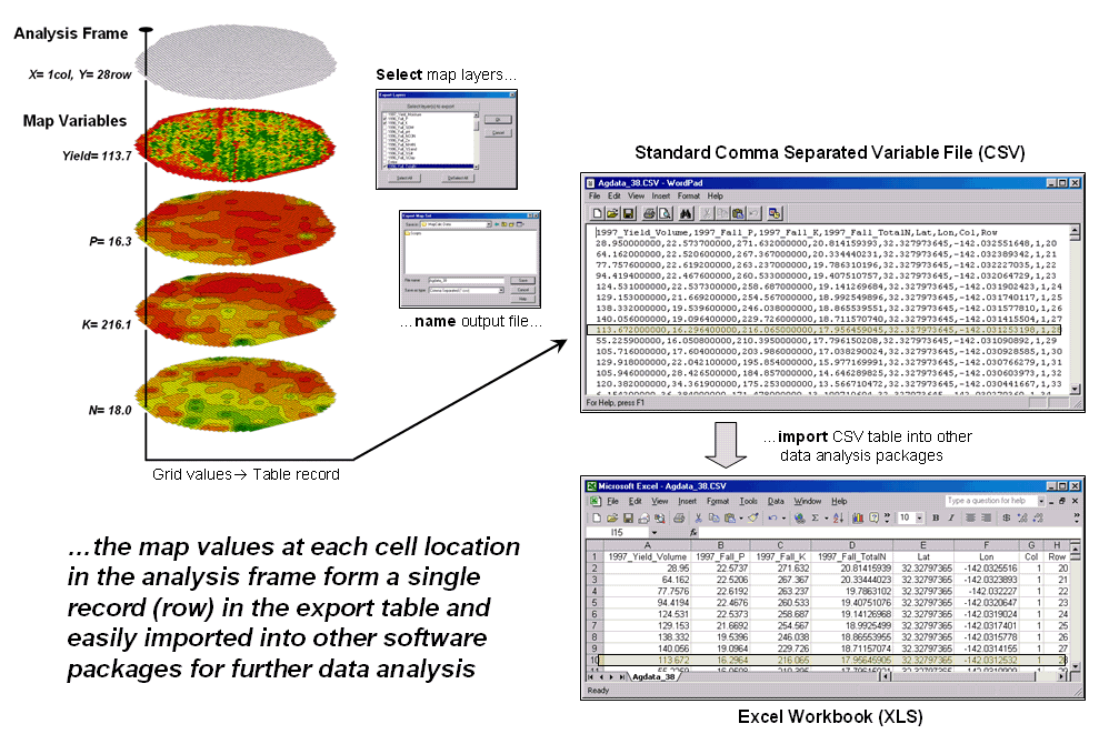 Figure 1. The
map values at each grid location form a single record in the exported table.
Figure 1. The
map values at each grid location form a single record in the exported table.
Figure 1 shows the process
for grid-based data. Recall that a
consistent analysis frame is used to organize the data into map layers. The map values at each cell location for selected
layers are reformatted into a single record and stored in a standard export
table that, in turn, can be imported into other data analysis software.
The example in the figure
shows the procedure for exporting a standard comma separated variable (CSV)
file with each record containing the selected data for a single grid cell. The user selects the map layers for export
and specifies the name of the output file.
The computer accesses the data and constructs a standard text line with
commas separating each data value. Note
that the column, row of the analysis frame and its latitude, longitude earth
poison is contained in each record. In
the example, the export file is brought into Excel for further processing.
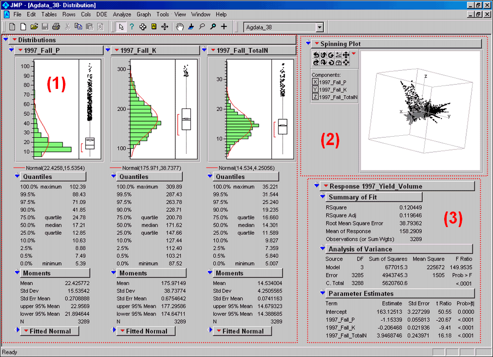 Figure
2. Mapped data can be imported into
standard statistical packages for further analysis.
Figure
2. Mapped data can be imported into
standard statistical packages for further analysis.
Figure 2 shows the agricultural
data imported into the JMP statistical package (by SAS). Area (1) shows the histograms and descriptive
statistics for the P, K and N map layers shown in figure 2. Area (2) is a “spinning 3D plot” of the data
that you can rotate to graphically visualize relationships among the map
layers. Area (3) shows the results of
applying a multiple linear regression model to predict crop yield from the soil
nutrient maps. These are but a few of
the tools beyond mapping that are available through data exchange between GIS
and traditional spreadsheet, database and statistical packages—a perspective
that integrates maps with other technologies.
Modern statistical packages
like JMP “aren’t your father’s” stat experience and are fully interactive with
point-n-click graphical interfaces and wizards to guide appropriate
analyses. The analytical tools, tables
and displays provide a whole new view of traditional mapped data. While a map picture might be worth a thousand
words, a gigabyte or so of digital map data is a whole revelation and foothold
for site-specific decisions.
Comparing
Yield Maps (return
to top)
One of the most fundamental operations in map analysis is the comparison of two maps. Questions like “how different are the maps?”, “how are they different?” and “where are they different?” immediately spring to mind. Quantitative answers are needed because visual comparison cannot fully consider all of the detail in an objective manner.
Recall
that there are two basic forms of mapped data used in precision farming—
discrete maps (vector) and map surfaces (grid).
Let’s consider discrete map comparison first. The two maps shown in figure 1 identify corn
yield for successive seasons on a central-pivot field in Colorado. Note that the maps have been normalized to
300 bu/ac and displayed with a common color pallet… but how different are they;
how are they different; and where are they different?
 Figure
1. Discrete Yield Maps for Consecutive
Years.
Figure
1. Discrete Yield Maps for Consecutive
Years.
While your eyes flit back and forth in an attempt to compare the maps, the computer approaches the problem more methodically. The first step converts the vector contour lines to a grid value for each cell. An analysis grid resolution is chosen (50ft cells are used in this example) and geometrically aligned with the maps. The dominant yield class within each cell is assigned its interval value (values 1 through 5 corresponding to the color range). The grid mesh used is superimposed on the yield maps for visual reference.
 Figure 2. Coincidence Map Identifying the Conditions
for Both Years.
Figure 2. Coincidence Map Identifying the Conditions
for Both Years.
The
next step, as shown in figure 2, combines the two maps into a single map that
indicates the “joint condition” for both years.
Since the two maps have identical gridding, the computer simply
retrieves the two class assignments for a grid location then converts them to a
single number.
The map-ematical procedure merely computes the “first value times ten plus the second value” to form a compound number. In the example shown in the figure, the value “forty-three” is interpreted as class 4 in the first year but decreasing to class 3 in the next year.
The
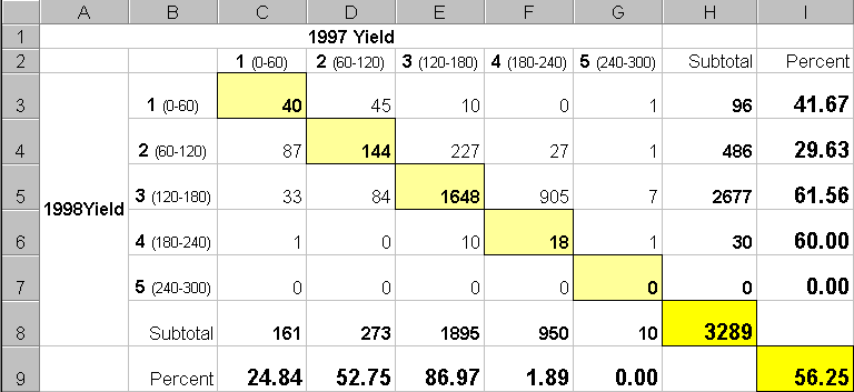
final step sums up the changes to generate a coincidence table (see figure
3). The columns and rows in the table
represent the class assignments on the 1997 and 1998 yield maps,
respectively. The body of the table
reports the number of cells for each joint condition. For example, column 4 and row 3 notes that
there are 905 occurrences where the yield class slipped from level four
(180-240bu/ac) to level three (120-180bu/ac).
 Figure
3. Coincidence Summary Table.
Figure
3. Coincidence Summary Table.
The
off-diagonal entries indicate changes between the two maps—the values indicate
the relative importance of the change.
For example, the 905 statistic for the “four-three” change is the
largest and therefore identifies the most significant change in the field. The 0 statistic for the “four-one”
combination indicates that level four never slipped clear to level 1.
The
diagonal entries summarize the agreement between the two maps. The greatest portion of the field that didn’t
change occurs for yield class 3 (“three-three” with 1640 cells). The statistic in the extreme lower-right
(56.25%) reports that only a little more than half the field didn’t change its
yield class.
Generally
speaking, the maps are very different (only 56.25% unchanged). The greatest difference occurred for class 4
(only 1.89% didn’t change). And a
detailed picture of the spatial patterns of change is depicted in the
coincidence map. That’s a lot more meat
in the answers to the basic map comparison questions (how much, how and where)
than visceral viewing can do. Next time
we’ll look at even more precise procedures for reporting the differences.
Comparing Yield Surfaces (return
to top)
Contour
maps are the most frequently used and familiar form of presenting precision ag
data. The color-coded ranges of yield
(0-60, 60-120, …etc. bushels) shown on the floor of the 3-D plots in figure 1
are identical to the discrete maps discussed in last month’s column. The color-coding of the contours is draped
for cross-reference onto the continuous 3-D surface of the actual data.
 Figure
1. 3-D Views of Yield Surfaces for
Consecutive Years.
Figure
1. 3-D Views of Yield Surfaces for
Consecutive Years.
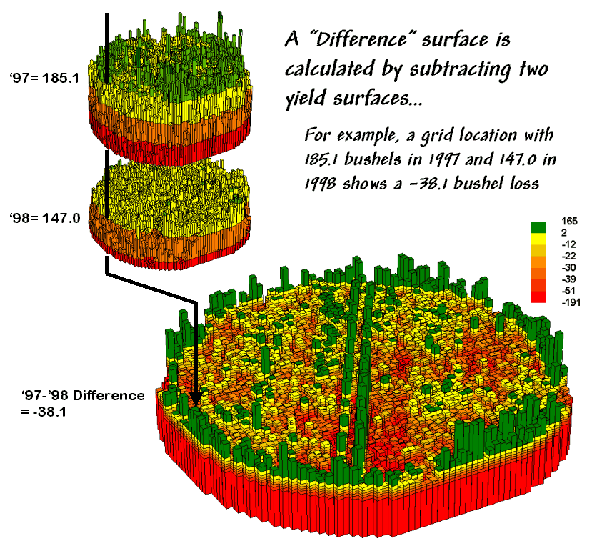
Note
the “spikes and pits” in the surfaces that graphically portray the variance in
yield data for each of the contour intervals.
While discrete map comparison identifies shifts in yield classes,
continuous surface comparison identifies the precise difference at each
location.
For
example, a yield value of 179 bushels and another one of 121 for successive
years are both assigned to the third contour interval (120 to180; yellow). A discrete map comparison would suggest that
no change in yield occurred for the location because the contour interval
remained constant. A continuous surface
comparison, on the other hand would report a fairly significant 58-bushel
decline.
 Figure
2. A Difference Surface Identifies the
Change in Yield.
Figure
2. A Difference Surface Identifies the
Change in Yield.
Figure
2 shows the calculations using the actual values for the same location
highlighted in the previous month’s discussion.
The discrete map comparison reported a decline from yield level 4 (180
to 240) to level 3 (120 to 180).
The
continuous surface comparison more precisely reports the change as –38.1
bushels. The differences for other 3,287
grid cells are computed to derive the Difference Surface that
tracks the subtle variations in the spatial pattern of the changes in
yield.
The
MapCalc command, “Compute Yield_98 minus Yield_97 for Difference” generates
the difference surface. If the simple
“map algebra” equation is expanded to “Compute (((Yield_98 minus Yield_97) /
Yield_97) *100)” a percent difference surface would be generated. Keep in mind that a map surface is merely a
spatially organized set of numbers that awaits detailed analysis then
transformation to generalized displays/summaries for human consumption.
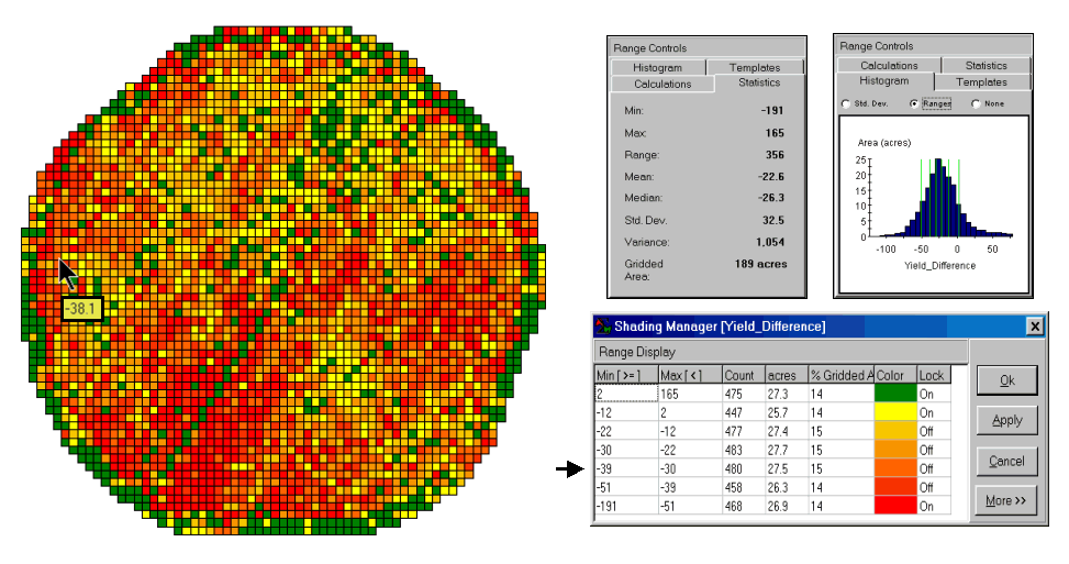
In
figure 2, note that the wildest differences (green spikes and red pits) occur
at the field edges and along the access road—from an increase of 165 bushels to
a decrease of 191 bushels. However,
notice that most of the change is about a 25-bushel decline (mean= -22.6;
median= -26.3) as denoted in figure 3.
 Figure
3. A 2-D Map and Statistics Describe the
Differences in Yield.
Figure
3. A 2-D Map and Statistics Describe the
Differences in Yield.
The
histogram of the yield differences shows the numerical distribution of the
data. Observe that it is normally
distributed and that the bulk of the data is centered about a 25-bushel
decline. The vertical lines in the
histogram locate the contour intervals used in the 2-D display that shows the
geographic distribution of the data.
The
detailed legend links the color-coding of the map intervals to some basic
frequency statistics. The example location
with the calculated decline of –38.1 is assigned to the –39 to –30 contour and
displayed as a mid-range red tone. The
display uses an Equal Count method with seven intervals, each
representing approximately 15% of the field.
Green is locked for the only interval of increased yield. The decreased yield intervals form a
color-gradient from yellow to red. All
in all, much more information in a more effective form than simply taping a
couple of yield maps to a wall for visual comparison.
The
ability to map-ematically evaluate continuous surfaces is fundamental to
precision farming. Difference surfaces
are one of the simplest and most intuitive forms. While the math and stat of other procedures
are fairly basic, the initial thought of “you can’t do that to a map” is
usually a reflection of our non-spatial statistics and paper-map legacies. In most instances, precision ag processing is
simply an extension of current practice from sample plots to mapped data. The remainder of this case study investigates
these extensions.
From Point Data to Map Surfaces (return
to top)
Soil
sampling has long been at the core of agricultural research and practice. Traditionally point-sampled data were
analyzed by non-spatial statistics to identify the “typical” level of a
nutrient throughout an entire field.
Considerable effort was expended to determine the best single estimate
and assess just how good it was in typifying a field.
However
none of the non-spatial techniques make use of the geographic patterns inherent
in the data to refine the estimate—the typical level is assumed every the same
within a field. The computed variance
(or standard deviation) indicates just how good this assumption is—the larger
the standard deviation the less valid is the assumption “everywhere the same.”
Surface
modeling, on the other hand, utilizes the spatial patterns in a data to
generate localized estimates throughout a field. Conceptually it “maps the variance” by using
geographic position to help explain the differences in sample values. In practice it simply fits a continuous
surface (kind of like a blanket) to the point data spikes.
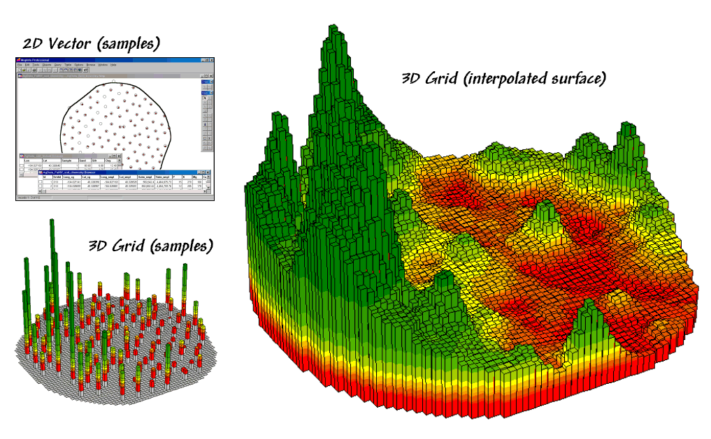 Figure 1. Spatial interpolation involves fitting a
continuous surface to sample points.
Figure 1. Spatial interpolation involves fitting a
continuous surface to sample points.
While
the extension from non-spatial to spatial statistics is quite a theoretical
leap, the practical steps are relatively easy.
The left side of figure 1 shows a point map of the phosphorous soil
samples. This highlights the principle
difference from traditional soil sampling—each sample must be geo-referenced
as it is collected. In addition, the sampling
pattern and intensity are often different to maximize spatial information
within the collected data (but that story is reserved for another time).
The
surface map on the right side of figure 1 depicts the continuous spatial
distribution derived from the point data.
Note that the high spikes in the western portion of the field and the
relatively low measurements in the center are translated into the peaks and
valleys of the surface map.
The
traditional, non-spatial approach, if mapped, would be a flat plane (average
phosphorous level) aligned within the bright yellow zone. Its “everywhere the same” assumption fails to
recognize the patterns of larger levels (greens) and smaller levels
(reds). A fertilization plan for
phosphorous based on the average level (22ppm) would be ideal for the yellow
zone but likely inappropriate for a lot of the field as the data vary from 5 to
102ppm.
It’s
common sense that nutrient levels vary throughout a field. However, there are four important
considerations before surface modeling is appropriate—
·
the pattern needs to be significant enough to warrant variable-rate
application (cost effective),
·
the prescription methods must be spatially appropriate for the pattern
(decision rules),
·
the derived map surface must fully reflect a real spatial pattern (map
accuracy), and
·
the procedure for generating the pattern must be straightforward and
easy to use (usability).
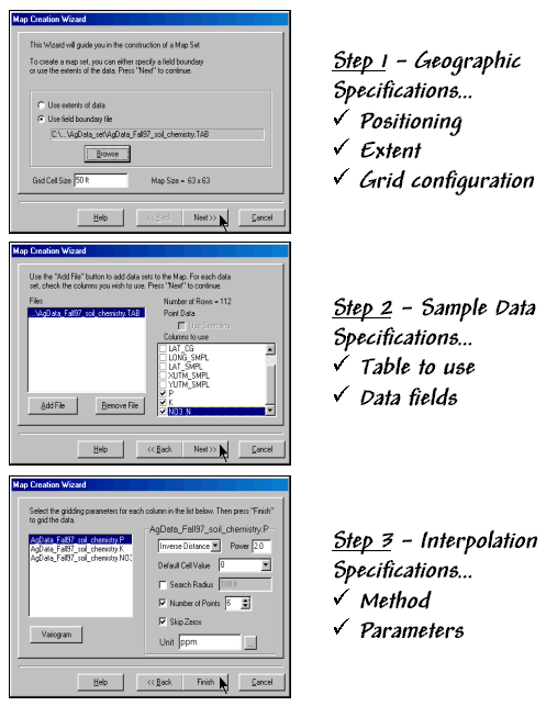 Figure 2. A Wizard interface guides a user through the
necessary steps for interpolating sample data.
Figure 2. A Wizard interface guides a user through the
necessary steps for interpolating sample data.
Let’s tackle the last point on usability first. The mechanics of generating an interpolated surface involves three steps to specify the geographic, data and interpolation considerations (see figure 2). The first step establishes the geographic position, field extent and grid configuration to be used. While these specifications can be made directly, it is easiest to simply reference an exiting map of the field boundary (positioning and extent—AgData_Fall97_soil_chemistry.TAB in this case) then enter the grid spacing to be used (configuration—50 feet).
The next step identifies the table and data fields to be used. The user navigates to the file (data table— AgData_Fall97_soil_chemistry.TAB) then simply checks the maps to be interpolated (data fields—P, K, NO3_N).
The final step establishes the interpolation method and necessary factors. In the example, the default Inverse Distance Squared (1/d2) method was employed using the six nearest sample points. Other methods, such as Krigging, could be specified and would result in somewhat different surfaces.
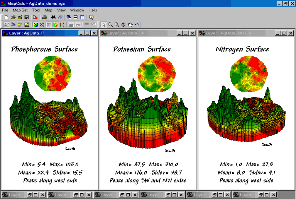 Figure 3. Interpolated Phosphorous, Potassium and
Nitrogen surfaces.
Figure 3. Interpolated Phosphorous, Potassium and
Nitrogen surfaces.
Figure
3 shows the P, K, NO3_N map surfaces that were generated by the Interpolation
Wizard specifications shown in figure 2.
The entire process including entering specifications, calculation of the
surfaces and display took less than a minute.
In
each instance the yellow zone contains the average for the entire field. Visually comparing the relative amounts and
patterns of the green and red areas gives you an idea of the difference between
the assumption that the average is everywhere and amount of spatial information
inherent in the soil sample data. Next
time we’ll investigate how to evaluate the accuracy of these maps—whether
they’re good maps or bad maps.
Benchmarking Interpolation Results (return
to top)
For
some, the previous discussion on generating maps from soil samples might have
been too simplistic—enter a few things then click on a data file and, viola,
you have a soil nutrient surface artfully displayed in 3D with a bunch of cool
colors draped all over it.
Actually,
it is that easy to create one. The
harder part is figuring out if it makes sense and whether it is something you
ought to use in analysis. The next few
columns will investigate how you can tell if the derived map is “a good map, or
a bad map.” This month we’ll assess the
relative amounts of spatial information provided in a whole-field average and
two different interpolated map surfaces.
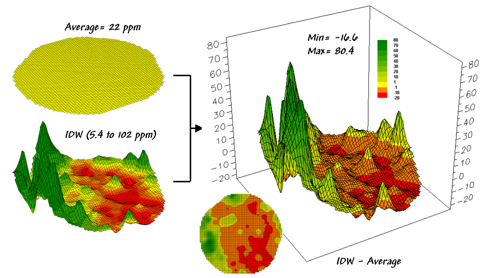 Figure 1. Spatial Comparison of a Whole-Field Average
and an IDW Interpolated Map.
Figure 1. Spatial Comparison of a Whole-Field Average
and an IDW Interpolated Map.
The top-left item in Figure 1 shows the map of
a field’s average phosphorous levels.
It’s not very exciting and looks like a pancake but that’s because there
isn’t any information about spatial variability in an average value—assumes
22ppm is everywhere in the field.
The
non-spatial estimate simply adds up all of the sample measurements and divides
by the number of samples to get 22ppm.
Since the procedure didn’t consider where the different samples were
taken, it can’t map the variations in the measurements. It thinks the average is everywhere, plus or
minus the standard deviation. But there
is no spatial guidance where phosphorous levels might be more, or where they
might be less.
The
spatially based estimates are shown in the map surface just below the
pancake. As described in the last
column, spatial interpolation looks at the relative positioning of the soil
samples as well as their measure phosphorous levels. In this instance the big bumps were
influenced by high measurements in that vicinity while the low areas responded
to surrounding low measurements.
The
map surface in the right portion of figure 1 objectively compares the two maps
simply by subtracting them. The colors
were chosen to emphasize the differences between the whole-field average
estimates and the interpolated ones. The
yellow band indicates the average level while the progression of green tones
locates areas where the interpolated map thought there was more
phosphorous. The progression of red
tones identifies the opposite with the average estimate being more than the
interpolated ones.
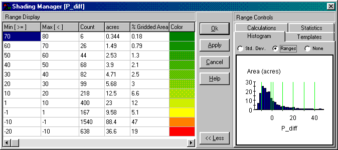 Figure 2.
Statistics summarizing the difference between the maps in figure 1.
Figure 2.
Statistics summarizing the difference between the maps in figure 1.
The
information in figure 2 shows that the difference between the two maps ranges
from –20 to +80ppm. If one assumes that
+/- 10ppm won’t significantly change a fertilization recommendation, then about
two-thirds (47+5.1+12= 64.1 percent of the field) is adequately covered by the
whole-field average. But that leaves
about a third of the field that is receiving too much (6.6+3+2.5+2.1+1.3+.79+.18=
16.5 percent) or too little (19 percent) phosphorous under a fertilization
program based on the average.
Now
turn your attention to figure 3 that compares maps derived by two different
interpolation techniques—IDW (inverse distance-weighted) and Krig. Note the similarity in the peaks and valleys
of the two surfaces. While subtle
differences are visible the general trends in the spatial distribution of the
data are identical.
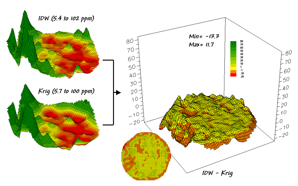 Figure 3. Spatial Comparison of IDW and Krig
Interpolated Maps.
Figure 3. Spatial Comparison of IDW and Krig
Interpolated Maps.
The
difference map on the right confirms the coincident trends. The broad band of yellow identifies areas
that are +/- 1 ppm. The brown color
identifies areas that are within 10 ppm with the IDW surface estimates a bit
more than the Krig ones. Applying the
same assumption about +/- 10 ppm difference being negligible in a fertilization
program the maps are effectively identical.
So
what’s the bottom line? That there are
substantial differences between a whole field average and interpolated
surfaces—at least for this data set. It
suggests that quibbling about the best interpolation technique isn’t as
important as using an interpolated surface (any surface) over the whole field
average. However, what needs to be
addressed is whether an interpolated surface (any surface) actually reflects
the real spatial distribution. That weighty
question awaits the next couple of columns.
Assessing Interpolation Performance (return
to top)
Last
month’s discussion compared the assumption of the field average with map
surfaces generated by two different interpolation techniques for phosphorous
levels throughout a field. While there was
considerable differences between the average and the derived surfaces (from -20
to +80ppm), there was relatively little difference between the two surfaces
(+/- 10ppm).
But
which surface best characterizes the spatial distribution of the sampled data? The answer to this question lies in Residual
Analysis—a technique that investigates the differences between estimated
and measured values throughout a field.
It’s common sense that one shouldn’t simply accept a soil nutrient map
without checking out its accuracy. Cool
graphics just isn’t enough.
Ideally,
one designs an appropriate sampling pattern and then randomly locates a number
of “test points” to assess interpolation performance. Since a lot is riding on the accuracy of the
interpolated maps, it makes sense to invest a little bit more just to see how
well things are going.
But
alas, that wasn’t the case in the AgData data base… nor is it in most
cases. One approach is to randomly
remove a small portion of the samples that will be withheld during
interpolation, then used to evaluate interpolated estimates.
 Figure 1.
Identifying a test set of samples.
Figure 1.
Identifying a test set of samples.
Figure
1 outlines a technique that uses Excel’s “random number generator” to select a test
set of samples. One specifies a
number range (1 to 112 for sample IDs), the number of samples desired (12 for a
10% sample) and the distribution for selecting numbers (“uniform” for an equal
chance of being selected). The table in
the middle of the figure identifies the twelve randomly selected sample points
that were eliminated from the interpolation data set and used to form the test
set.
The
constrained set data was used to generate two map surfaces of phosphorous. The map on the left in figure 2 used the
default specifications for Inverse Distance Weighted (IDW), while the one on
the right used Kriging defaults. A
common color palette from red (0-10ppm) through green (100-110ppm) was applied
to both. The yellow inflection zone
encompasses the whole-field average phosphorous level.
 Figure 2.
Interpolated IDW and Krig surfaces based on the constrained data set.
Figure 2.
Interpolated IDW and Krig surfaces based on the constrained data set.
Both
maps display a similar shape but there are some subtle differences. The Krig surface appears generally smoother
and the IDW surface has four distinct peaks in the northeast portion of the
field (right side). Otherwise the
surfaces seem fairly similar as they were for the full set of data discussed
last month.
But
which surface did a better job at estimating the measured phosphorous levels in
the test set? The table in figure 3
reports the results. The first column
identifies the sample ID and the second column the actual measured value for
that location.
 Figure 3.
Residual Analysis table assessing interpolation performance.
Figure 3.
Residual Analysis table assessing interpolation performance.
Column
C simply depicts estimating the whole-field average (21.6) at each of the test
locations. Column D computes the
difference of the “estimate minus actual”—formally termed the residual. For example, the first test point (ID#59)
estimated average of 21.6 but was measured as 20.0 so the residual is 1.6
(21.6-20.0= 1.6ppm)… not bad. However,
test point #109 is way off (21.6-103.0= -81.4ppm)… nearly 400% error!
The
residuals for the IDW and Krig maps are similarly calculated to form columns R
and H, respectively. First note that the
residuals for the whole-field average are generally larger than either those
for the IDW or Krig estimates. Next note
that the residual patterns between the IDW and Krig are very similar—when one
is way off, so is the other and usually by about the same amount. A notable exception is for test point #91
where Krig dramatically over-estimates.
The
rows at the bottom of the table summarize the residual analysis results. The “Residual sum” row characterizes any bias
in the estimates—a negative value indicates a tendency to underestimate with
the magnitude of the value indicating how much.
The –92.8 value for the whole-field average indicates a relatively
strong bias to underestimate.
The
“Average error” row reports how far off on the average each estimate was. The 19.0ppm figure is three times worse than
Krig’s estimated error (6.08) and nearly four times worse than IDW’s
(5.24). Comparing the figures to the
assumption that a +/-10ppm is negligible in a fertilization program it is
readily apparent that the whole-field estimate is inappropriate to use and that
the accuracy differences between IDW and Krig are minor.
The
“Normalized error” row simply calculates the average error as a proportion of
the average value for the test set of samples (5.24/29.3= .18 for IDW). This index is the most useful as it allows
you to compare the relative map accuracies between different maps. Generally speaking, maps with normalized
errors of more than .10 are very suspect and one might not want to make
important decisions using them.
So
what’s the bottom line? Residual
Analysis is an important component of precision agriculture. Without an understanding of the relative
accuracy and interpolation error of the base maps, one can’t be sure of the
recommendations derived from the data.
The investment in a few extra
sampling points for testing and residual analysis of these data provides
a sound foundation for site-specific management. Without it, the process becomes one of blind
faith.
Calculating Similarity Within A Field (return to top)
How often have you seen a precision ag presenter “lasso” a portion of a map with a laser pointer and boldly state “See how similar this area is to the locations over here and here” as the pointer rapidly moves about the map. More often than not, there is a series of side-by-side maps serving as the background scenery for the laser show.
But just how similar is one field location to another? Really similar, or just a little similar? And just how dissimilar are all of the other areas? While visceral analysis can identify broad relationships it takes a quantitative map analysis approach to handle the detailed scrutiny demanded by site-specific management.
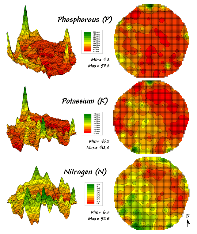 Figure 1. Map surfaces identifying the spatial distribution
of P,K and N throughout a field.
Figure 1. Map surfaces identifying the spatial distribution
of P,K and N throughout a field.
Consider the three maps shown in figure 1— what areas identify similar patterns? If you focus your attention on a location in the southeastern portion how similar are all of the other locations?
The answer to these questions are much too complex for visual analysis and certainly beyond the geo-query and display procedures of standard desktop mapping packages. The data in the example shows the relative amounts of phosphorous, potassium and nitrogen throughout a central pivot corn field in Colorado.
In visual analysis you move your focus among the maps to summarize the color assignments at different locations. The difficulty in this approach is two-fold— remembering the color patterns and calculating the difference. Quantitative map analysis does the same thing except it uses map values in place of colors. In addition, the computer doesn’t tire as easily as you and completes the comparison for all of the locations throughout the map window (3289 grid cells in this example) in a couple seconds.
The upper-left portion of figure 2 illustrates capturing the data patterns of two locations for comparison. The “data spear” at map location 45column, 18row identifies the P-level as 11.0, the K-level as 177.0 and N-level as 32.9ppm. This step is analogous to your eye noting a color pattern of burnt-red, dark-orange and light-green. The other location for comparison (32c, 62r) has a data pattern of P= 53.2, K= 412.0 and N= 27.9. Or as your eye sees it, a color pattern of dark-green, dark-green and yellow.
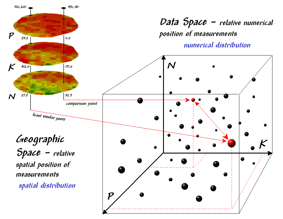 Figure 2. Conceptually linking geographic space and
data space.
Figure 2. Conceptually linking geographic space and
data space.
The right side of figure 2 conceptually depicts how the computer calculates a similarity value for the two response patterns. The realization that mapped data can be expressed in both geographic space and data space is key to understanding quantitative analysis similarity.
Geographic space uses coordinates, such latitude and longitude, to locate things in the real world—such as the southeast and extreme north points identified in the example field. The geographic expression of the complete set of measurements depicts their spatial distribution in familiar map form.
Data space, on the other hand, is a bit less familiar. While you can’t stroll through data space you can conceptualize it as a box with a bunch of balls floating within it. In the example, the three axes defining the extent of the box correspond to the P, K and N levels measured in the field. The floating balls represent grid locations defining the geographic space—one for each grid cell. The coordinates locating the floating balls extend from the data axes—11.0, 177.0 and 32.9 for the comparison point. The other point has considerably higher values in P and K with slightly lower N (values 53.2, 412.0, 27.9 respectively) so it plots at a different location in data space.
The bottom line for data space analysis is that the position of a point identifies its numerical pattern—low, low, low in the back-left corner, while high, high, high is in the upper-right corner of the box. Points that plot in data space close to each other are similar; those that plot farther away are less similar.
In the example, the floating ball closest to you is least similar (greatest distance) from the comparison point. This distance becomes the reference for “most different” and sets the bottom value of the similarity scale (0% similar). A point with an identical data pattern plots at exactly the same position in data space resulting in a data distance of 0 that equates to the highest similarity value (100% similar).
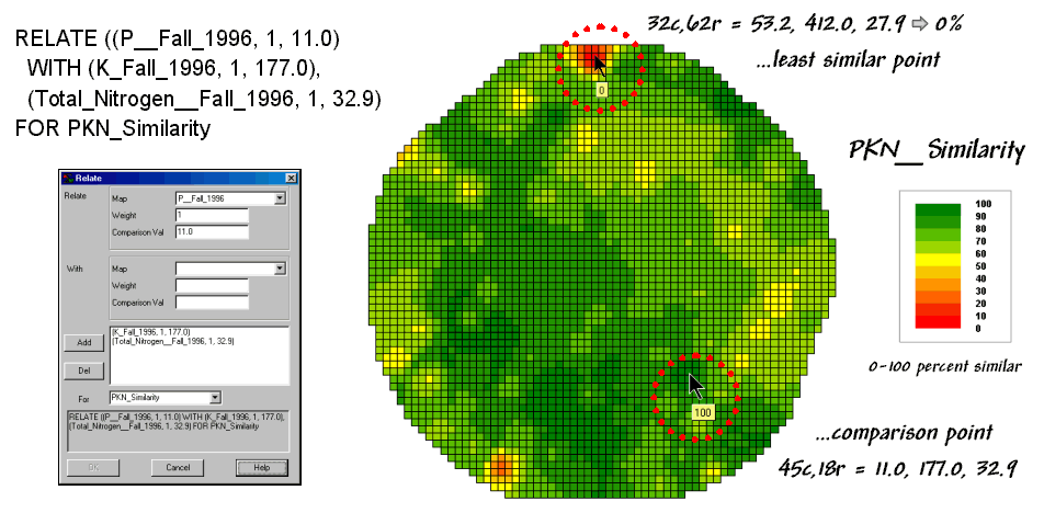 Figure 3. A similarity map identifying how related
locations are to a given point.
Figure 3. A similarity map identifying how related
locations are to a given point.
The similarity map shown in figure 3 applies the similarity scale to the data distances calculated between the comparison point and all of the other points in data space. The green tones indicate field locations with fairly similar P, K and N levels to the comparison location in the field—with the darkest green identifying locations with identical P, K and N levels. The red tones indicate increasing dissimilar areas. It is interesting to note that most of the very similar locations are in the western portion of the field.
A similarity map can be an invaluable tool for investigating spatial patterns in any complex set of mapped data. While humans are unable to conceptualize more than three variables (the data space box), a similarity index can handle any number of input maps. Also, the different layers can be weighted to reflect relative importance in determining overall similarity.
In effect, a similarity map replaces a lot of laser-pointer waving and subjective suggestions of similar/dissimilar areas with a concrete, quantitative measurement at each map location. The technique moves map analysis well beyond the old “I’d never have seen, it if I hadn’t believe it” mode of spatial interpretation.
Identifying Data Zones (return to top)
Last section introduced the concept of “data distance” as a means to measure similarity within a map. One simply mouse-clicks a location and all of the other locations are assigned a similarity value from 0 (zero percent similar) to 100 (identical) based on a set of specified maps. The statistic replaces difficult visual interpretation of map displays with an exact quantitative measure at each location.
An extension to the technique allows you to circle an area then compute similarity based on the typical data pattern within the delineated area. In this instance, the computer calculates the average value within the area for each map layer to establish the comparison data pattern, then determines the normalized data distance for each map location. The result is a map showing how similar things are to the area of interest.
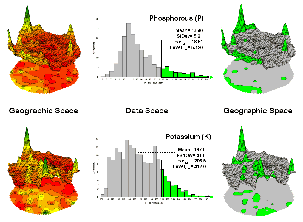 Figure 1. Identifying areas of unusually high
measurements.
Figure 1. Identifying areas of unusually high
measurements.
The link between Geographic Space and Data Space is key. As shown in figure 1, spatial data can be viewed as a map or a histogram. While a map shows us “where is what,” a histogram summarizes “how often” measurements occur (regardless where they occur).
The top-left portion of the figure shows a 2D/3D map display of the relative amount of phosphorous (P) throughout a farmer’s field. Note the spikes of high measurements along the edge of the field, with a particularly big spike in the north portion.
The histogram to the right of the map view forms a different perspective of the data. Rather than positioning the measurements in geographic space it summarizes their relative frequency of occurrence in data space. The X-axis of the graph corresponds to the Z-axis of the map—amount of phosphorous. In this case, the spikes in the graph indicate measurements that occur more frequently. Note the high occurrence of phosphorous around 11ppm.
Now to put the geographic-data space link to use. The shaded area in the histogram view identifies measurements that are unusually high—more than one standard deviation above the mean. This statistical cutoff is used to isolate locations of high measurements as shown in the map on the right. The procedure is repeated for the potassium (K) map surface to identify its locations of unusually high measurements.
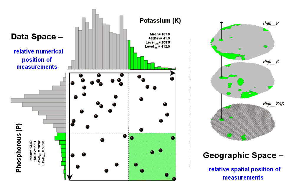 Figure 2. Identifying joint coincidence in both data
and geographic space.
Figure 2. Identifying joint coincidence in both data
and geographic space.
Figure 2 illustrates combining the P and K data to locate areas in the field that have high measurements in both. The graphic on the left is termed a scatter diagram or plot. It graphically summarizes the joint occurrence of both sets of mapped data.
Each ball in the scatter plot schematically represents a location in the field. Its position in the plot identifies the P and K measurements at that location. The balls plotting in the shaded area of the diagram identify field locations that have both high P and high K. The upper-left partition identifies joint conditions in which neither P nor K are high. The off-diagonal partitions in the scatter plot identify locations that are high in one but not the other.
The aligned maps on the right show the geographic solution for areas that are high in both of the soil nutrients. A simple map-ematical way to generate the solution is to assign 1 to all locations of high measurements in the P and K map layers (bight green). Zero is assigned to locations that aren’t high (light gray). When the two binary maps (0/1) are multiplied, a zero on either map computes to zero. Locations that are high on both maps equate to 1 (1*1 = 1). In effect, this “level-slice” technique maps any data pattern you specify… just assign 1 to the data interval of interest for each map variable.
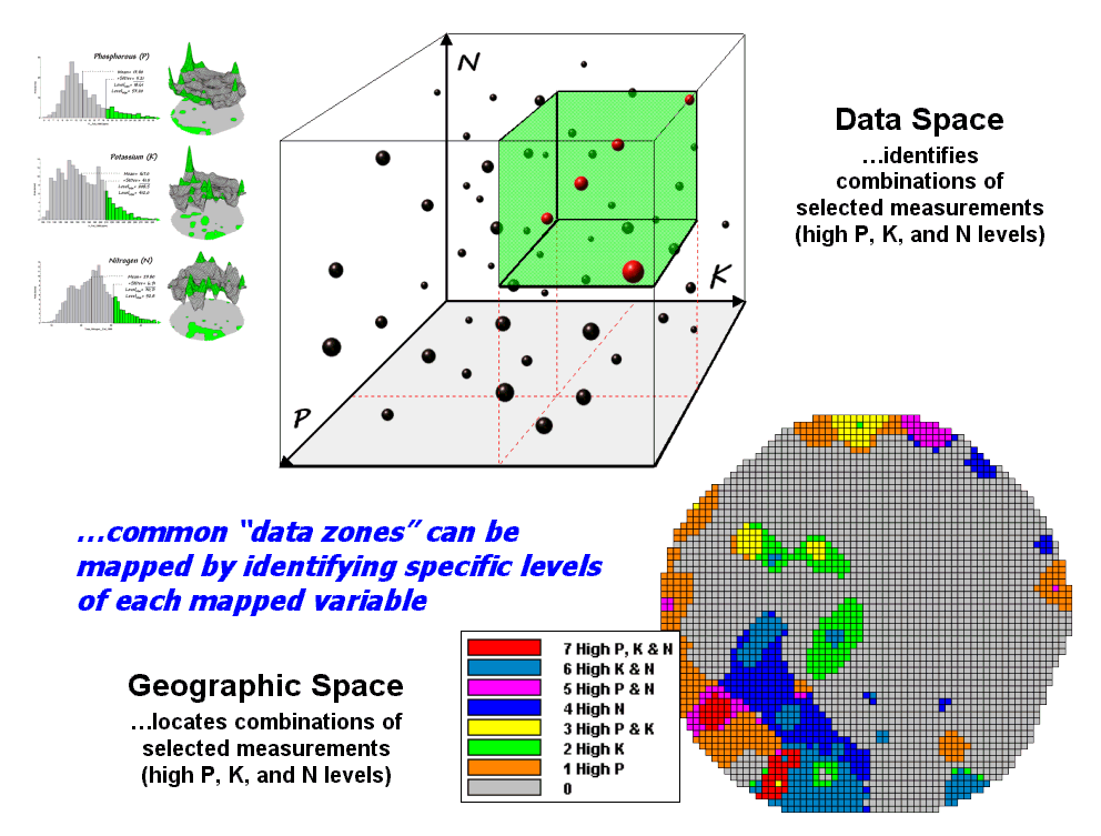 Figure 3. Level-slice classification using three map
variables.
Figure 3. Level-slice classification using three map
variables.
Figure 3 depicts level slicing for areas that are unusually high in P, K and N (nitrogen). In this instance the data pattern coincidence is a box in 3-dimensional scatter plot space.
However a map-ematical trick was employed to get the map solution shown in the figure. On the individual maps, high areas were set to P=1, K= 2 and N=4, then the maps were added together.
The result is a range of coincidence values from zero (0+0+0= 0; gray= no high areas) to seven (1+2+4= 7; red= high P, high K, high N). The map values in between identify the map layers having high measurements. For example, the yellow areas with the value 3 have high P and K but not N (1+2+0= 3). If four or more maps are combined, the areas of interest are assigned increasing binary progression values (…8, 16, 32, etc)—the sum will always uniquely identify the combinations.
While level-slicing isn’t a very sophisticated classifier, it does illustrate the useful link between data space and geographic space. This fundamental concept forms the basis for most geostatistical analysis… including map clustering and regression to be tackled in the next couple of sections.
Mapping Data Clusters (return
to top)
The last couple of topics have focused on analyzing data similarities within a stack of maps. The first technique, termed Map Similarity, generates a map showing how similar all other areas are to a selected location. A user simply clicks on an area and all other map locations are assigned a value from 0 (0% similar—as different as you can get) to 100 (100% similar—exactly the same data pattern).
The other technique, Level Slicing, enables a user to specify a data range of interest for each map in the stack then generates a map identifying the locations meeting the criteria. Level Slice output identifies combinations of the criteria met—from only one criterion (and which one it is), to those locations where all of the criteria are met.
While both of these techniques are useful in examining spatial relationships, they require the user to specify data analysis parameters. But what if you don’t know what Level Slice intervals to use or which locations in the field warrant Map Similarity investigation? Can the computer on its own identify groups of similar data? How would such a classification work? How well would it work?
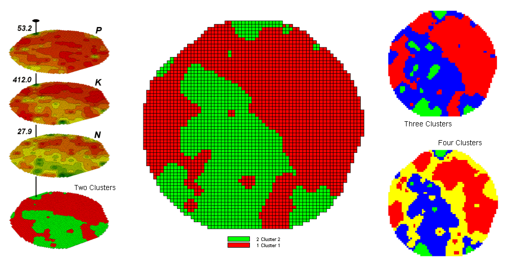 Figure 1. Examples of Map Clustering.
Figure 1 shows some examples derived from Map Clustering. The “floating” maps on the left show the input map stack used for the cluster analysis. The maps are the same P, K, and N maps identifying phosphorous, potassium and nitrogen levels throughout a cornfield that were used for the examples in the previous topics.
The map in the center of the figure shows the results of classifying the P, K and N map stack into two clusters. The data pattern for each cell location is used to partition the field into two groups that are 1) as different as possible between groups and 2) as similar as possible within a group. If all went well, any other division of the field into two groups would be not as good at balancing the two criteria.
The two smaller maps at the right show the division of the data set into three and four clusters. In all three of the cluster maps red is assigned to the cluster with relatively low responses and green to the one with relatively high responses. Note the encroachment on these marginal groups by the added clusters that are formed by data patterns at the boundaries.
The mechanics of generating cluster maps are quite simple. Simply specify the input maps and the number of clusters you want then miraculously a map appears with discrete data groupings. So how is this miracle performed? What happens inside cluster’s black box?
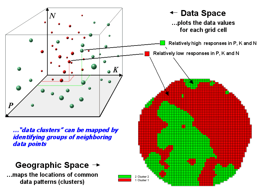 Figure 2. Data patterns for map locations are depicted
as floating balls in data space.
Figure 2. Data patterns for map locations are depicted
as floating balls in data space.
The schematic in figure 2 depicts the process. The floating balls identify the data patterns for each map location (geographic space) plotted against the P, K and N axes (data space). For example, the large ball appearing closest to you depicts a location with high values on all three input maps. The tiny ball in the opposite corner (near the plot origin) depicts a map location with small map values. It seems sensible that these two extreme responses would belong to different data groupings.
The specific algorithm used in clustering was discussed in a previous topic (see “Clustering Map Data”, Topic 4, Precision Farming Primer). However for this discussion, it suffices to note that “data distances” between the floating balls are used to identify cluster membership—groups of balls that are relatively far from other groups and relatively close to each other form separate data clusters. In this example, the red balls identify relatively low responses while green ones have relatively high responses. The geographic pattern of the classification is shown in the map at the lower right of the figure.
Identifying groups of neighboring data points to form clusters can be tricky business. Ideally, the clusters will form distinct “clouds” in data space. But that rarely happens and the clustering technique has to enforce decision rules that slice a boundary between nearly identical responses. Also, extended techniques can be used to impose weighted boundaries based on data trends or expert knowledge. Treatment of categorical data and leveraging spatial autocorrelation are other considerations.
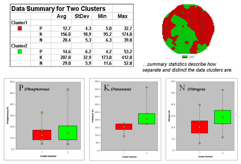 Figure 3.
Clustering results can be roughly evaluated using basic statistics.
Figure 3.
Clustering results can be roughly evaluated using basic statistics.
So how do know if the clustering results are acceptable? Most statisticians would respond, “you can’t tell for sure.” While there are some elaborate procedures focusing on the cluster assignments at the boundaries, the most frequently used benchmarks use standard statistical indices.
Figure 3 shows the performance table and box-and-whisker plots for the map containing two clusters. The average, standard deviation, minimum and maximum values within each cluster are calculated. Ideally the averages would be radically different and the standard deviations small—large difference between groups and small differences within groups.
Box-and-whisker plots enable us to visualize these differences. The box is centered on the average (position) and extends above and below one standard deviation (width) with the whiskers drawn to the minimum and maximum values to provide a visual sense of the data range. When the diagrams for the two clusters overlap, as they do for the phosphorous responses, it tells us that the clusters aren’t very distinct along this axis. The separation between the boxes for the K and N axes suggests greater distinction between the clusters. Given the results a practical PF’er would likely accept the classification results… and statisticians hopefully will accept in advance my apologies for such a conceptual and terse treatment of a complex topic.
Predicting Maps (return
to top)
Talk about the future of precision Ag… how about maps of things yet to come? Sounds a bit far fetched but Spatial Data Mining is taking us in that direction. For years non-spatial statistics has been predicting things by analyzing a sample set of data for a numerical relationship (equation) then applying the relationship to another set of data. The drawbacks are that the non-approach doesn’t account for geographic relationships and the result is just a table of numbers addressing an entire field.
Extending predictive analysis to mapped data seems logical. After all, maps are just organized sets of numbers. And the GIS toolbox enables us to link the numerical and geographic distributions of the data. The past several columns have discussed how the computer can “see” spatial data relationships— “descriptive techniques” for assessing map similarity, classification units and data zones. The next logical step is to apply “predictive techniques” to generate extrapolative maps.
If fact, the first time I used prediction mapping was in 1991 to extend a test market project for a phone company. The customer’s address was used to geo-code sales of a new product that enabled two numbers with distinctly different rings to be assigned to a single phone— one for the kids and one for the parents. Like pushpins on a map, the pattern of sales throughout the city emerged with some areas doing very well, while in other areas sales were few and far between.
The demographic data for the city was analyzed to calculate a prediction equation between product sales and census block data. The prediction equation derived from the test market sales in one city was applied to another city by evaluating exiting demographics to “solve the equation” for a predicted sales map. In turn the predicted map was combined with a wire-exchange map to identify switching facilities that required upgrading before release of the product in the new city.
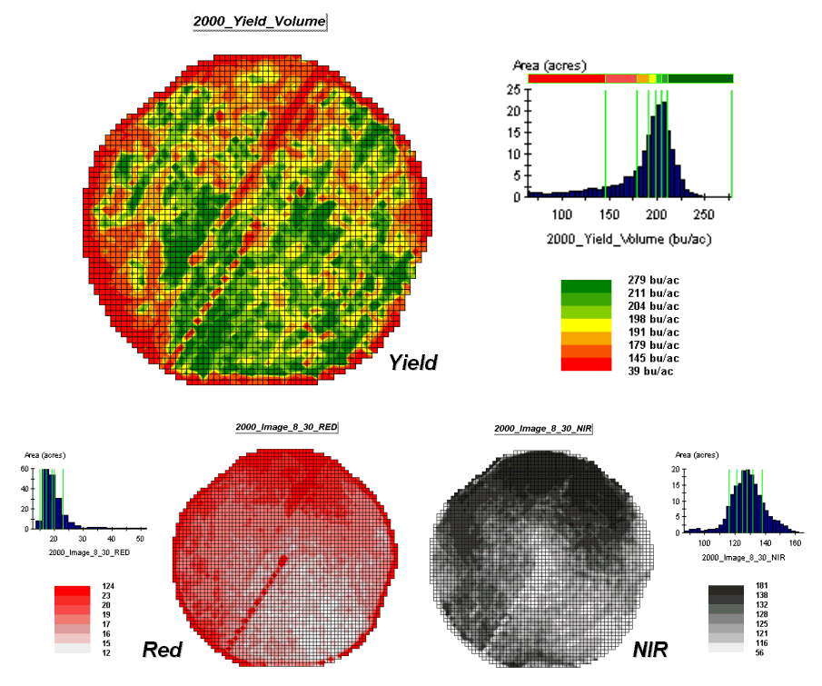 Figure
1. The corn yield map (top) identifies
the pattern to predict; the red and near-infrared maps (bottom) are used to
build the spatial relationship.
Figure
1. The corn yield map (top) identifies
the pattern to predict; the red and near-infrared maps (bottom) are used to
build the spatial relationship.
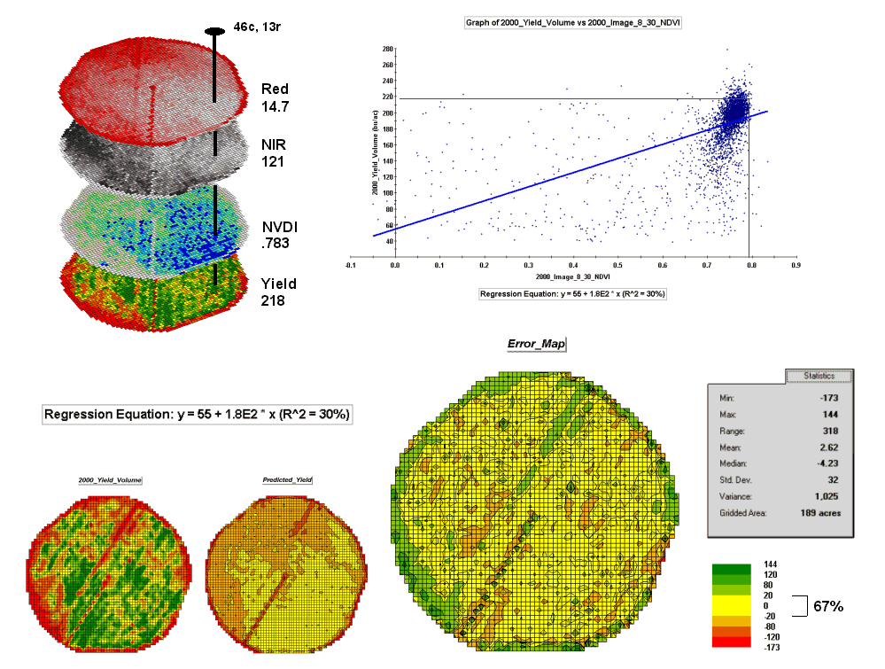
To illustrate the data mining procedure, the approach can be applied to the cornfield data that has been focus for the past several columns. The top portion of figure 1 shows the yield pattern for the field varying from a low of 39 bushels per acre (red) to a high of 279 (green). Corn yield, like “sales yield,” is termed the dependent map variable and identifies the phenomena we want to predict.
The independent map variables depicted in the bottom portion of the figure are used to uncover the spatial relationship— prediction equation. In this instance, digital aerial imagery will be used to explain the corn yield patterns. The map on the left indicates the relative reflectance of red light off the plant canopy while the map on the right shows the near-infrared response (a form of light just beyond what we can see).
While it is difficult for you to assess the subtle relationships between corn yield and the red and near-infrared images, the computer “sees” the relationship quantitatively. Each grid location in the analysis frame has a value for each of the map layers— 3,287 values defining each geo-registered map covering the 189-acre field.
 Figure
2. The joint conditions for the spectral
response and corn yield maps are summarized in the scatter plots shown on the
right.
Figure
2. The joint conditions for the spectral
response and corn yield maps are summarized in the scatter plots shown on the
right.
For example, top portion of figure 2 identifies that the example location has a “joint” condition of red equals 14.7 counts and yield equals 218 bu/ac. The red lines in the scatter plot on the right show the precise position of the pair of map values—X= 14.7 and Y= 218. Similarly, the near-infrared and yield values for the same location are shown in the bottom portion of the figure.
In fact the set of “blue dots” in both of the scatter plots represents data pairs for each grid location. The blue lines in the plots represent the prediction equations derived through regression analysis. While the mathematics is a bit complex, the effect is to identify a line that “best fits the data”— just as many data points above as below the line.
In a sense, the line sort of identifies the average yield for each step along the X-axis (red and near-infrared responses respectively). Come to think of it, wouldn’t that make a reasonable guess of the yield for each level of spectral response? That’s how a regression prediction is used… a value for red (or near-infrared) in another field is entered and the equation for the line is used to predict corn yield. Repeat for all of the locations in the field and you have a prediction map of yield from an aerial image… but alas, if it were only that simple and exacting.
A major problem is that the “r-squared” statistic for both of the prediction equations is fairly small (R^^2= 26% and 4.7% respectively) which suggests that the prediction lines do not fit the data very well. One way to improve the predictive model might be to combine the information in both of the images. The “Normalized Density Vegetation Index (NDVI)” does just that by calculating a new value that indicates relative plant vigor— NDVI= ((NIR – Red) / (NIR + Red)).
Figure 3 shows the process for calculating NDVI for the sample grid location— ((121-14.7) / (121 + 14.7))= 106.3 / 135.7= .783. The scatter plot on the right shows the yield versus NDVI plot and regression line for all of the field locations. Note that the R^^2 value is a higher at 30% indicating that the combined index is a better predictor of yield.
 Figure
3. The red and NIR maps are combined for
NDVI value that is a better predictor of yield.
Figure
3. The red and NIR maps are combined for
NDVI value that is a better predictor of yield.
The bottom portion of the figure evaluates the prediction equation’s performance over the field. The two smaller maps show the actual yield (left) and predicted yield (right). As you would expect the prediction map doesn’t contain the extreme high and low values actually measured.
However the larger map on the right calculates the error of the estimates by simply subtracting the actual measurement from the predicted value at each map location. The error map suggests that overall the yield “guesses” aren’t too bad— average error is a 2.62 bu/ac over guess; 67% of the field is within 20 bu/ac. Also note that most of the over estimating occurs along the edge of the field while most of the under estimating is scattered along curious NE-SW bands.
While evaluating a prediction equation on the data that generated it isn’t validation, the procedure provides at least some empirical verification of the technique. It suggests a glimmer of hope that with some refinement the prediction model might be useful in predicting yield before harvest. Next month we’ll investigate some of these refinement techniques and see what information can be gleamed by analyzing the error surface.
Stratifying Maps for Better Predictions (return
to top)
The last section described procedures for predictive analysis of mapped data. While the underlying theory, concerns and considerations can easily consume a graduate class for a semester the procedure is quite simple. The grid-based processing preconditions the maps so each location (grid cell) contains the appropriate data. The “shishkebab” of numbers for each location within a stack of maps are analyzed for a prediction equation that summarizes the relationships.
In the example discussed in the last section, regression analysis was used to relate a map of NDVI (“normalized density vegetation index” derived from remote sensing imagery) to a map of corn yield for a farmer’s field. Then the equation was used to derive a map of predicted yield based on the NDVI values and the results evaluated for how well the prediction equation performed.
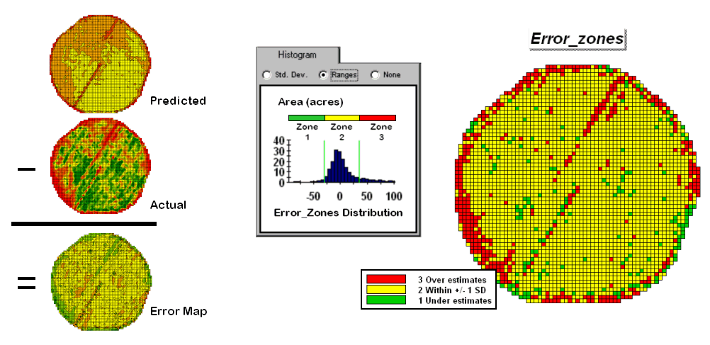 Figure 1. A
field can be stratified based on prediction errors.
Figure 1. A
field can be stratified based on prediction errors.
The
left side of figure 1 shows the evaluation procedure. Subtracting the actual yield values from the
predicted ones for each map location derives an Error Map. The previous discussions noted that the yield
“guesses” weren’t too bad—average error of 2.62 bu/ac with 67% of the estimates
within 20 bu/ac of the actual yield.
However, some locations were as far off as 144 bu/ac (over-guess) and
–173 bu/ac (under-guess).
One
way to improve the predictions is to stratify the data set by
breaking it into groups of similar characteristics. The idea is that set of prediction equations
tailored to each stratum will result in better predictions than a single
equation for an entire area. The
technique is commonly used in non-spatial statistics where a data set might be
grouped by age, income, and/or education prior to analysis. In spatial statistics additional factors for
stratifying, such as neighboring conditions and/or proximity, can be used.
While
there are several alternatives for stratifying, subdividing the error map will
serve to illustrate the conceptual approach.
The histogram in the center of figure 1 shows the distribution of values
on the Error Map. The vertical bars
identify the breakpoints at plus/minus one standard deviation and divide the
map values into three strata—zone 1 of unusually high under-guesses (red), zone
2 of typical error (yellow) and zone 3 of unusually high over-guesses
(green). The map on the right of the
figure locates the three strata throughout the field.
The
rationale behind the stratification is that the whole-field prediction equation
works fairly well for zone 2 but not so well for zones 1 and 3. The assumption is that conditions within zone
1 makes the equation under estimate while conditions within zone 3 cause it to
over estimate. If the assumption holds
one would expect a tailored equation for each zone would be better at predicting
than an overall equation. Figure 2
summarizes the results of deriving and applying a set of three prediction
equations.
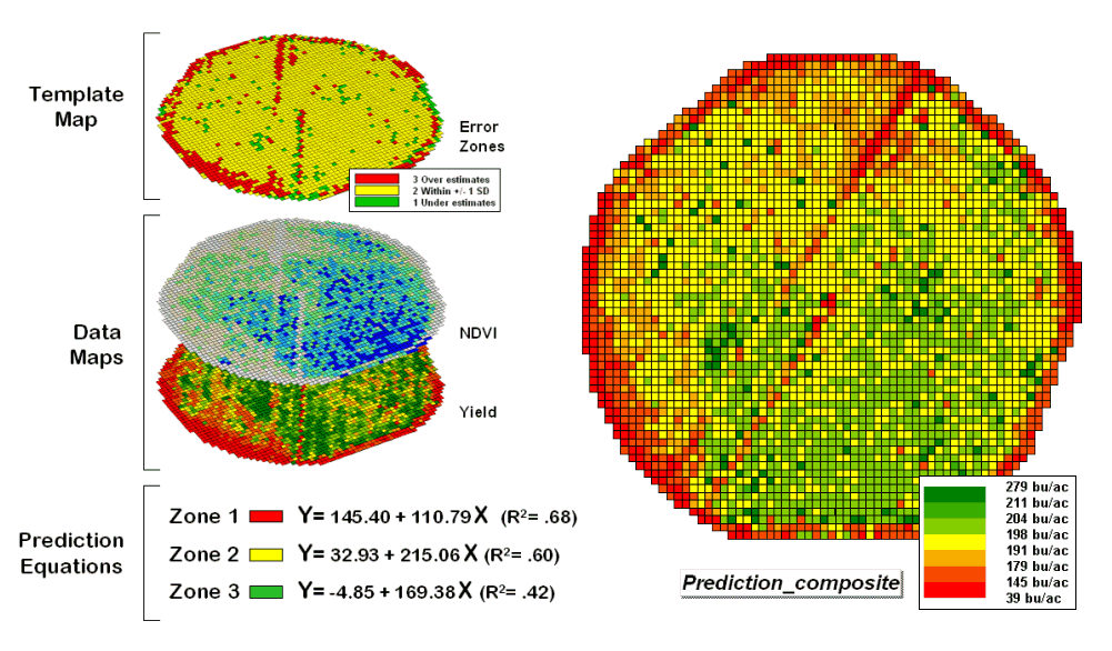 Figure 2.
After stratification, prediction equations can be derived for each
element.
Figure 2.
After stratification, prediction equations can be derived for each
element.
The
left side of the figure illustrates the procedure. The Error Zones map is used as a
template to identify the NDVI and Yield values used to calculate three separate
prediction equations. For each map
location, the algorithm first checks the value on the Error Zones map
then sends the data to the appropriate group for analysis. Once the data has been grouped a regression
equation is generated for each zone. The
“r-squared” statistic for all three equations (.68, .60, and .42 respectively)
suggests that the equations fit the data fairly well and ought to be good
predictors. The right side of figure 2
shows the composite prediction map generated by applying the equations to the
NDVI data respecting the zones identified on the template map.
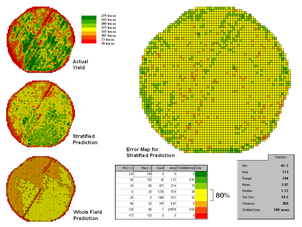 Figure 3.
Stratified and whole-field predictions can be compared using statistical
techniques.
Figure 3.
Stratified and whole-field predictions can be compared using statistical
techniques.
The
left side of figure 3 provides a visual comparison between the actual yield and
predicted maps. The “stratified
prediction” shows detailed estimates that more closely align with the actual
yield pattern than the “whole-field” derived prediction map. The error map for the stratified prediction
shows that eighty percent of the estimates are within +/- 20 bushels per
acre. The average error is only 4 bu/ac
with maximum under and over-estimates of –81.2 and 113, respectively. All in all, not bad guessing of yield based
on a remote sensing shot of the field nearly a month before the field was
harvested.
A
couple of things should be noted from this example of spatial data mining. First, that there is a myriad of other ways
to stratify mapped data—1) Geographic Zones, such as proximity to the field
edge; 2) Dependent Map Zones, such as areas of low, medium and high yield; 3)
Data Zones, such as areas of similar soil nutrient levels; and 4) Correlated
Map Zones, such as micro terrain features identifying small ridges and
depressions. The process of identifying
useful and consistent stratification schemes is an emerging research frontier
in the spatial sciences.
Second,
the error map is key in evaluating and refining the prediction equations. This point is particularly important if the
equations are to be extended in space and time.
The technique of using the same data set to develop and evaluate the prediction
equations isn’t always adequate. The
results need to be tried at other locations and dates to verify
performance. While spatial data mining
methodology might be at hand, good science is imperative.
The bottom line is that maps are increasingly
seen as organized sets of data that can be map-ematically analyzed for spatial
relationships… we have only scratched the surface. The applications of spatial analysis and data
mining in production agriculture are in their infancy. As the agricultural sciences embrace spatial
technology, research will tailor the procedures for the unique data and
situations facing farmers.
The
Precision Farming Primer is intended to spark this revolution… the wildfire of change
will come from the agronomists, soil scientists, crop consultants, equipment
dealers, chemical distributors and innovative farmers. The effect will be farmland management more
in tune with the spatial patterns within fields. The result will be improved management
practices that increase productivity while reducing environmental
problems. While the trappings of precision
agriculture might appear unfamiliar (and even uncomfortable) at the onset, the
technology will soon become second nature like those of the previous
“mechanical” and “green” revolutions that preceded it.
Spatial Analysis
Operations (return
to top)
Grid-based map analysis involves two broad categories of
operations—Spatial Statistics and Spatial Analysis. Table 4-1 outlines some of the specific
techniques within each category. Spatial
Statistics tools, like the ones presented in the previous discussions 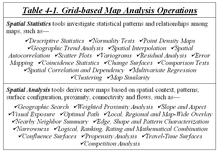 on comparing maps, interpolation, data
grouping and predictive models, respond to “numerical” relationships in mapped
data.
on comparing maps, interpolation, data
grouping and predictive models, respond to “numerical” relationships in mapped
data.
Spatial Analysis tools, on the other hand, investigate “contextual” relationships, such as slope/aspect, buffers, effective proximity, optimal path, visual exposure and shape analysis. Rather than statistical investigation of mapped data relationships, these techniques examine geographic patterns, vicinity characteristics and connectivity among features.
From this perspective, four classes of spatial analysis techniques can be identified that— reclassify map categories, overlay two or more maps, measure distance and connectivity, and characterize cartographic neighborhoods.
In the broadest sense, Reclassification operations merely repackage existing information on a single map. Overlay operations, on the other hand, involve two or more maps and result in the delineation of new information. Distance operations generate entirely new information by characterizing the relative positioning of map features. Neighborhood operations summarize the conditions occurring in the general vicinity of a location.
Figure 7-1. A Distance tool can be used to buffer
special features in the field.
While precision agriculture often involves spatial statistics in its
applications, most other GIS applications focus on spatial analysis operations,
particularly the “geo-query” capability to retrieve locations of map features
stored in a database.
For example, a forester might want to identify forest parcels of Douglas fir on
Cohasset soil within a county. Or a real
estate agent might query the residential listing for houses within a specified
distant of a school and costing less than $300,000.
_____________________
Author’s note: An educational version of the MapCalc software by Red Hen Systems used in the case study provides “hands-on” exercises for the topics discussed in this Case Study series. See www.redhensystems.com for more information and ordering; US$21.95 for Student CD and US$495.00 for Instructor CD with multi-seat license for a computer lab (prices subject to change).
______________