Beyond Mapping III
|
Map
Analysis book with companion CD-ROM
for hands-on exercises and further reading |
Behind the
Scenes of Virtual Reality — discusses
the basic considerations and concepts in 3d-object rendering
How to
Rapidly Construct a Virtual Scene — describes
the procedures in generating a virtual scene from landscape inventory
data
How to
Represent Changes in a Virtual Forest — discusses
how simulations and "fly-bys" are used to visualize landscape changes
and characteristics
Capture "Where and
When" on Video-based GIS — describes
how
Video Mapping Brings Maps
to Life — describes
how video maps are generated and discusses some applications of video mapping
<Click here>
right-click to download a printer-friendly version of this topic (.pdf).
(Back to the Table of
Contents)
______________________________
Behind the Scenes of Virtual Reality
(GeoWorld, June 2000, pg. 22-23)
Over the past three decades,
cutting-edge
The transition of
This evolution is most apparent in
multimedia
While these visualizations are dramatic, none of the multimedia
Since discovery of herbal dyes, the color pallet has been a dominant part of
mapping. A traditional map of forest
types, for example, associates various colors with different tree species—red
for ponderosa pine, blue for Douglas fir, etc.
Cross-hatching or other cartographic techniques can be used to indicate
the relative density of trees within each forest polygon. A map’s legend relates the abstract colors
and symbols to a set of labels identifying the inventoried conditions. Both the map and the text description are
designed to conjure up a vision of actual conditions and the resulting spatial
patterns.
The map has long served as an abstract summary while the landscape artist’s
canvas has served as a more realistic rendering of a scene. With the advent of computer maps and virtual
reality techniques the two perspectives are merging. In short, color pallets are being replaced by
rendering pallets.
Like the artist’s painting, complete objects are grouped into patterns rather
than a homogenous color applied to large areas.
Object types, size and density reflect actual conditions. A sense of depth is induced by plotting the
objects in perspective. In effect, a virtual
reality
Fundamental to the process is the ability to design realistic objects. An effective approach, termed geometric
modeling, utilizes an interface (figure 32-1) similar to a 3-D computer-aided
drafting system to construct individual scene elements. A series of sliders and buttons are used to
set the size, shape, orientation and color of each element comprising an
object. For example, a tree is built by
specifying a series of levels representing the trunk, branches, and
leaves. Level one forms the trunk that
is interactively sized until the designer is satisfied with the representation. Level two establishes the pattern of the
major branches. Subsequent levels
identify secondary branching and eventually the leaves themselves.
Figure 32-1. Designing tree objects.
The basic factors that define each
level include 1) linear positioning, 2) angular positioning, 3) orientation, 4)
sizing and 5) representation. Linear
positioning determines how often and where branches occur. In fig. 1, the major branching occurs part
way up the trunk and is fairly evenly spaced.
The angular positioning, sets how often branches occur around the trunk or
branch to which it is attached. The
branches at the third level in the figure form a fan instead of being equally
distributed around the branch.
Orientation refers to how the branches are tilting. Note that the lower branches droop down from
the trunk, while the top branches are more skyward looking. The third-order branches tend show a similar
drooping effect in the lower branches.
Sizing defines the length and taper a particular
branch. In the figure, the lower
branches are considerably smaller than the mid-level branches. Representation covers a lot of factors
identifying how a branch will appear when it is displayed, such as its
composition (a stick, leaf or textured crown), degree of randomness, and 24-bit
Figure 32-2. The inset on the left shows
various branching patterns. The inset on
the right depicts the sequencing of four branching levels.
Figure 32-2 illustrates some branching patterns and levels used to
construct tree-objects. The tree
designer interface at first might seem like overkill—sort of a glorified
“painting by the numbers.” While it’s
useful for the artistically-challenged, it is critical for effective 3-D
rendering of virtual landscapes.
The mathematical expression of an object allows the computer to generate a
series of “digital photographs” of a representative tree under a variety of
look-angles and sun-lighting conditions.
The effect is similar to flying around the tree in a helicopter and
taking pictures from different perspectives as the sun moves across the
sky. The background of each bitmap is
made transparent and the set is added to the library of trees. The result is a bunch of snapshots that are
used to display a host of trees, bushes and shrubs under different viewing
conditions.
The object-rendering process results in a “palette” of objects analogous to the
color palette used in conventional
_______________________
How to Rapidly Construct a Virtual
Scene
(GeoWorld, July 2000, pg. 22-23)
The previous column described how 3-dimensional objects, such as trees,
are built for use in generating realistic landscape renderings. The drafting process uses an interface that
enables a user to interactively adjust the trunk’s size and shape then add branches
and leaves with various angles and positioning.
The graphic result is similar to an artist’s rendering of an individual
tree.
The digital representation, however, is radically different. Because it is a mathematically defined
object, the computer can generate a series of “digital photographs” of the tree
under a variety of look-angles and sun-lighting conditions. The effect is similar to flying around the
tree in a helicopter and taking pictures from different perspectives as the sun
moves across the sky.
The background of each of these snapshots is made transparent and the set is
added to a vast library of tree symbols.
The result is a set of pictures that are used to display a host of
trees, bushes and shrubs under different viewing conditions. A virtual reality scene of a landscape is
constructed by pasting thousands of these objects in accordance with forest
inventory data stored in a
Figure 32-3. Basic steps
in constructing a virtual reality scene.
There are six steps in constructing
a fully rendered scene (see Figure 32-3).
A digital terrain surface provides the lay of the landscape. The
The link between the
Figure 32-4. Forest inventory data
establishes tree types, stocking density and maturity.
Finally, information on percent
maturity establishes the baseline height of the tree. In a detailed tree library several different
tree objects are generated to represent the continuum from immature, mature and
old growth forms. Figure 32-4 shows the
tree exam files for two polygons identified in the adjacent graphic. The first column of values identifies the
tree symbol (library ID#). Polygon 1573
has 21 distinct tree types including snags (dead trees). Polygon 1658 is much smaller and only
contains 16 different types. The second
column indicates the percent maturity while the third defines the number of
trees. These data shown are for an
extremely detailed U.S. Forest Service research area in
Once the appropriate tree symbol and number of trees are identified the
computer can begin “planting” them. This
step involves determining a specific location within the polygon and sizing the
snapshot based on the tree’s distance from the viewpoint. Most often trees are randomly placed however
clumping and compaction factors can be used to create clustered patterns if
appropriate.
Figure 32-5. Tree symbols are “planted” then
sized depending on their distance from the viewpoint.
Tree sizing is similar pasting and
resizing an image in a word document.
The base of the tree symbol is positioned at the specific location then
enlarged or reduced depending on how far the tree is from the viewing position. Figure 32-5 shows a series of resized tree
symbols “planted” along a slope—big trees in front and progressively smaller
ones in the distance.
The process of rendering a scene is surprisingly similar to that of landscape
artist. The terrain is painted and
landscape features added. In the
artist’s world it can take hours or days to paint a scene. In virtual reality the process is completed
in a minute or two as hundreds of trees are selected, positioned and resized
each second.
Since each tree is embedded on a transparent canvas they obscure what is behind
them—textured terrain and/or other trees, depending on forest stand and viewing
conditions. Terrain locations that are
outside of the viewing window or hidden behind ridges are simply ignored. The multitude of issues and extended
considerations surrounding virtual reality’s expression of
_______________________
How to Represent Changes in a
Virtual
(GeoWorld, August 2000, pg. 24-25)
The previous columns described the
steps in rendering a virtual landscape.
The process begins with a 3D drafting program used to construct
mathematical representations of individual scene elements similar to a
painter’s sketches of the different tree types that occur within an area. The tree library is linked to
The result is a strikingly lifelike rendering of the landscape instead of a
traditional map. While maps use colors
and abstract symbols to represent forest conditions, the virtual forest uses
realistic scene elements to reproduce the composition and structure of the
forest inventory data. This lifelike 3D
characterization of spatial conditions extends the boundaries of mapping from
dry and often confusing drawings to more familiar graphical perspectives.
32-6. Changes in the
landscape can be visualized by modifying the forest inventory data.
The baseline rendering for a data
set can be modified to reflect changes on the landscape. For example, the top two inserts in figure
32-6 depict a natural thinning and succession after a severe insect
infestation. The winter effects were
introduced by rendering with a snow texture and an atmospheric haze.
The lower pair of inserts show the before and after views of
a proposed harvest block. Note
the linear texture features in the clearcut that
identify the logging road. Alternative
harvest plans can be rendered and their relative visual impact assessed. In addition, a temporal sequence can be
generated that tracks the ‘green-up” through forest growth models as a
replanted parcel grows. In a sense, the
baseline
While
Figure
32-7. A “fly-by” movie is constructed by generating
a sequence of renderings then viewing them in rapid succession (click here to view the fly-by).
Admittedly, real-time “fly-bys” of
While trees off in the distance form a modeled texture, placement differences
of a couple of feet for trees in the foreground can significantly alter a
scene. For key viewpoints
Figure 32-8. Strikingly real snapshots of
forest data can be generated from either limited or robust
Realistic trees, proper placement, appropriate under-story textures and
shaded relief combine to produce strikingly real snapshots of a landscape. In robust, forest inventory data the
rendering closely matches reality.
However, equally striking results can be generated from limited
data. For example, the “green” portions
on topographic maps indicate forested areas, but offer no information about
species mixture, age/maturity or stocking.
Within a
That brings up an important point as map display evolves to virtual reality—how
accurate is the portrayal? Our
cartographic legacy has wrestled with spatial and thematic accuracy, but
“rendering fidelity” is an entirely new concept (figure 32-8). Since you can’t tell by looking, standards
must be developed and integrated with the metadata accompanying a
rendering. Interactive links between the
underlying data and the snapshot are needed.
Without these safeguards, it’s “viewer beware” and opens a whole new
avenue for lying with maps.
While Michael Creighton’s emersion into a virtual representation of a database
(the novel Disclosure) might be decades off, virtual renderings of
_______________________
Capture "Where and When" on Video-based GIS
(GeoWorld, September 2000, pg. 26-27)
The past three columns described
procedures for translating
An alternative is to populate a
Video mapping is an exciting part of the revolution in visualization of mapped
data. It records
With video mapping, the construction of a multimedia
During the Recording Step, video mapping encodes
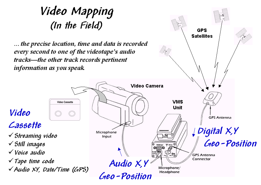
Figure 32-9. Video Mapping
in the Field. As video
is recorded, the precise location, time, and date are recorded every second to
one of the videotape’s audio tracks. The
other track records pertinent information as you speak.
In turn, the acoustic signals are sent to one of the audio channels through
the microphone input connector on the video camera. The result is recording the
The direct recording of “where and
when” on the tape greatly facilitates field data collection—as long as there is
Most contemporary video cameras have a switch between photo and movie
mode. In movie mode, streaming video is
recorded at 30 frames per second. In
photo mode, the camera acts like a still camera and "freezes" the
frame for several seconds as it records the image to videotape. In this mode, a one-hour videotape can record
over 500 digital pictures. In both photo
and movie modes the one-second
The Indexing Step involves connecting
the video mapping unit to a computer and playing the video (see figure
32-10). In this configuration, the audio
cord is switched to the Headphone Output connector and a second cable is
connected to the Lan C connector on the camera. The connector provides information on tape
position (footage on older cameras and time code on newer ones) used in
indexing and playback control of the tape similar to those on a standard
Figure 32-10. Indexing the
Videotape. The
video, audio notes and
As the videotape is played, the audio X,Y and
time code information is sent to the video mapping unit where it is converted
to digital data and sent to the serial port on the computer. If a headset was used in the field, the voice
recording on the second audio channel is transferred as well.
For indexing there are five types of information available—streaming video
(movie mode), still images (photo mode), voice audio (headset), tape time code
(tape position), and
Video mapping software records the
The Review Step uses the indexed database to access audio and video information
on the tape. The hardware configuration
is the same as for indexing (audio, Lan
C and serial cables). Clicking on any
indexed location retrieves its
Map features can start applications, open files and display images. The software works with video capture cards
to create still images and video clips you can link to map features, giving
maximum flexibility in choosing a data review method. In many applications the completed multimedia
map is exported as an HTML file for viewing with any browser or over the
Internet. The map features can contain
any or all five of the basic
information types:
ü Text —
interpreted from audio as .
ü Data —
interpreted from audio as .DAT, .XLS or .DBF file
ü Audio —
captured as .WAV file (about 100KB per 5 seconds)
ü Image —
captured as .JPG file (about 50KB per image)
ü Video —
captured as .
_______________________
Video Mapping Brings Maps to Life
(GeoWorld, October 2000, pg. 24-25)
As detailed in last month’s column, video mapping enables anyone with a
computer and video camera to easily create their own interactive video
maps. The integration of computers,
video camera, and
For example, corridor mapping of oil and gas pipelines, transmission towers,
right of ways and the like provide images of actual conditions not normally
part of traditional maps. In law
enforcement, video mapping can be used from reconnaissance to traffic safety to
forensics. Agriculture applications
include crop scouting, weed/pest management, verification of yield maps, and
“as-applied” mapping. Geo-business uses
range from conveying neighborhood character, to insurance reporting to web page
development.
By coupling audio/visual information to other
Data is collected without a computer in the field or cumbersome additional
equipment. Figure 32-11 shows the VMSTM
unit by Red Hen Systems (see author’s note) that weighs less than a pound and
is connected to the video camera via a small microphone cable. The
Figure
32-11. Video Mapping Hardware.
The VMS 200 unit enables recording and processing of
The office configuration consists of
a video camera, VMS unit, notebook or desktop computer, and mapping
software. The software generates a map
automatically from the data recorded on the videotape. Once a map is created, it can be personalized
by placing special feature points that relate to specific locations. These points are automatically or manually
linked to still images, video clips, sound files, documents, data sets, or
other actions that are recalled at the touch of a button. A voice recognition package is under
development that will create free-form text and data-form entry. The mapping software also is compatible with
emerging
While a map is being created, or at a later time, a user can mark special
locations with a mouse-click to "capture" still images, streaming
video or audio files. The “fire wire”
port on many of the newer computers makes capturing multimedia file a snap. Once captured, a simple click on the map
feature accesses the images, associated files, or video playback beginning at
that location.
Sharing or incorporating information is easy because the video maps are
compatible with most
popular
Differential post-processing is another important software addition. The post-processing software (EZdiffTM) takes base station correction data
from the Internet and performs a calculation against the video mapped
Figure 32-12 shows an example of the
video mapping software. The dark blue
line on map identifies the route of an ultralite (a
hang-glider with an engine). Actually
the line is composed of a series of dots— one for each second the video camera
was recording. Clicking anywhere on the
line will cause the camera, or
The light blue and red dots in the figure are feature locations where still
images, audio tracks and video clips were captured to the hard disk. The larger inset is a view of the lake and
city from the summit of a hiking trail.
The adjacent red dots are a series of similar images taken along the
trail. When a video camera is set in
photo mode, a one-hour videotape contains nearly 600 exposures— no film,
processing or printing required. In
addition, the automatic assignment of
Figure
32-12. Video Mapping Software.
Specialized software builds a linked database and provides numerous
features for accessing the data, customizing map layout and exporting to a
variety of formats.
The top captured image on the right
side of the figure shows a photo taken from an ultralite
inventory of bridges along a major highway.
The middle image is a field photo of cabbage loper
damage in a farmer’s field. The bottom
image is of a dummy in a training course for police officers. The web pages for these and other
applications are online for better understanding of video mapping capabilities
(see author’s notes).
For centuries, maps have been
abstractions of reality that use inked lines, symbols and shadings to depict
the location of physical features and landscape conditions. Multimedia
_______________________
Author's
Note: the information contained in this column is intended
to describe the conceptual approach, considerations and practical applications
of video mapping. Several online
demonstrations of this emerging technology in a variety of applications are
available at http://www.redhensystems.com. For information on the information on the VMS
200TM Video Mapping System contact Red Hen Systems, Inc, 2310 East
Prospect Road, Suit A, Fort Collins, USA 80525,
Phone: (800) 237-4182, Email: info@redhensystems.com, Web site:
http://www.redhensystems.com/.
(Back to the Table of Contents)