The following description of map analysis operations is from the pMAP User’s Manual, Computer-Assisted Map Analysis (chapter 3), Spatial Information Systems, Inc., Fort Collins, Colorado, 1993; Chapter written by Joseph K. Berry. "Hands-on" experience with the operations described is available with the Tutorial Map Analysis Package (tMAP). The material is discussed in greater detail in the books Beyond Mapping and Spatial Reasoning .
MAP ANALYSIS CAPABILITIESThe development of a generalized analytic structure for map processing is similar to those of many other non-spatial systems. For example, most data base packages contain less than twenty analytic operations, yet may be used to create models for such diverse applications as address lists, payroll, inventory control, or commitment accounting. Once developed, these logical data base commands are fixed into menus for easy end-user applications.
A flexible analytic structure provides for dynamic simulation as well as data base management. For example, a typical spreadsheet package allows users to define interrelationships among variables. A financial model of a company's production process may be established by specifying a logical sequence of primitive operations and map variables. By changing specific values of the model, the impact of several fiscal scenarios can be simulated. Data base management and spreadsheet packages have revolutionized the handling of non-spatial data. The potential of computer-assisted map analysis promises a similar revolution for spatial data processing.
From this perspective, four classes of primitive operations can be identified. Those which
Reclassification operations merely repackage existing information on a single map. Overlay operations, on the other hand, involve two or more maps and result in the delineation of new boundaries. Distance and connectivity operations generate entirely new information by characterizing the juxta-positioning of features. Neighborhood operations summarize the conditions occurring in the general vicinity of a location. The reclassifying and overlaying operations based on point processing are the backbone of current GIS applications, allowing rapid updating and examination of mapped data. However, other than the significant advantage of speed and ability to handle tremendous volumes of data, these capabilities are similar to those of manual processing. The map-wide overlays, distance and neighborhood operations identify more advanced analytic capabilities.
RECLASSIFYING MAPSThe first, and in many ways the most fundamental class of analytical operations, involves the reclassification of map categories. Each operation involves the creation of a new map by assigning thematic values to the categories of an existing map. These values may be assigned as a function of the initial value, the position, the contiguity, the size, or the shape of the spatial configuration of the individual categories. Each of the reclassification operations involves the simple repackaging of information on a single map, and results in no new boundary delineations. Such operations can be thought of as the purposeful "recoloring" of maps.
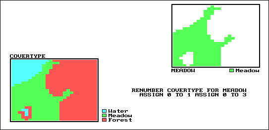
Figure 1 shows the result of simply reclassifying a map as a function of its initial thematic values. For display, a unique symbol is associated with each value. In the figure, the COVERTYPE map has categories of Open Water, Meadow and Forest. These features are stored as thematic values 1, 2 and 3, respectively, and displayed as separate graphic patterns. A binary map that isolates the meadow can be created by simply assigning 0 to the open and forested areas, and displaying the graphic symbol " " (blank) wherever this value occurs.
A similar reclassification operation might involve the ranking or weighing of qualitative map categories to generate a new map with quantitative values. A map of soil types, for example, might be assigned values that indicate the relative suitability of each soil type for residential development. Quantitative values may also be reclassified to yield new quantitative values. This might simply involve a specified reordering of map categories (e.g., given a map of soil moisture content, generate a map of suitability levels for plant growth). Or, it could involve the application of a generalized reclassifying function, such as "level slicing," which splits a continuous range of map category values into discrete intervals (e.g., derivation of a contour map from a map of topographic elevation values).
 |
| Figure 1. Reclassification of map categories can be based on initial thematic value, as in this example. The COVERTYPES of open water and forest are renumbered to the value zero which is displayed as a blank. The resulting map isolates the MEADOW region. |
Other quantitative reclassification functions include a variety of arithmetic operations involving map category values and a specified or computed constant. Among these operations are addition, subtraction, multiplication, division, exponentiation, maximization, minimization, normalization and other scalar mathematical and statistical operators. For example, a map of topographic elevation expressed in feet may be converted to meters by multiplying each map value by the appropriate conversion factor of 3.28083 feet per meter.
Reclassification operations can also relate to location, as well as purely thematic attributes associated with a map. One such characteristic is position. An overlay category represented by a single "point" location, for example, might be reclassified according to its latitude and longitude. Similarly, a line segment or areal feature could be reassigned values indicating its center or general orientation.
A related operation, termed parceling, characterizes category contiguity. This procedure identifies individual "clumps" of one or more points having the same numerical value and spatially contiguous (e.g., generation of a map identifying each lake as a unique value from a generalized water map representing all lakes as a single category).
Another location characteristic is size. In the case of map categories associated with linear features or point locations, overall length or number of points might be used as the basis for reclassifying those categories. Similarly, an overlay category associated with a planar area might be reclassified according to its total acreage or the length of its perimeter. For example, an overlay of surface water might be reassigned values to indicate the area of individual lakes or the length of stream channels. The same sort of technique might also be used to deal with volume. Given a map of depth to bottom for a group of lakes, for example, each lake might be assigned a value indicating total water volume based on the areal extent of each depth category.
In addition to the value, position, contiguity, and size of features, shape characteristics may also be used as the basis for reclassifying map categories. Categories represented by point locations have measurable "shapes" insofar as the set of points imply linear or areal forms (i.e., just as stars imply constellations). Shape characteristics associated with linear forms identify the patterns formed by multiple line segments (e.g., dendritic stream pattern). The primary shape characteristics associated with areal forms include feature integrity, boundary convexity, and nature of edge.
Feature integrity relates to "intact-ness" of an area. A category that is broken into numerous "fragments" and/or contains several interior "holes" is said to have less spatial integrity than ones without such violations. Feature integrity can be summarized as the Euler Number that is computed as the number of holes within a feature less one short of the number of fragments which make up the entire feature. An Euler Number of zero indicates features that are spatially balanced, whereas larger negative or positive numbers indicate less spatial integrity.
The other characteristics of shape, convexity and edge, relate to the configuration of boundaries of areal features. Convexity is the measure of the extent to which an area is enclosed by its background, relative to the extent to which the area encloses this background. The Convexity Index for a feature is computed by the ratio of its perimeter to its area. The most regular configuration is that of a circle which is totally convex and, therefore, not enclosed by the background at any point along its boundary. Comparison of a feature's computed convexity to a circle of the same area, results in a standard measure of boundary regularity. The nature of the boundary at each point can be used for a detailed description of boundary configuration. At some locations the boundary might be an entirely concave intrusion, whereas others might be at entirely convex protrusions. Depending on the "degree of edginess," each point can be assigned a value indicating the actual boundary convexity at that location.
This explicit use of cartographic shape as an analytic parameter is unfamiliar to most GIS users. However, a non-quantitative consideration of shape is implicit in any visual assessment of mapped data. Particularly promising is the potential for applying quantitative shape analysis techniques in the areas of digital image classification and wildlife habitat modeling. A map of forest stands, for example, might be reclassified such that each stand is characterized according to the relative amount of forest edge with respect to total acreage and the frequency of interior forest canopy gaps. Those stands with a large proportion of edge and a high frequency of gaps will generally indicate better wildlife habitat for many species.
OVERLAYING OPERATIONS
Operations for overlaying maps begin to relate to spatial coincidence, as well as to the thematic nature of cartographic information. The general class of overlay operations can be characterized as "light-table gymnastics." These involve the creation of a new map on which the value assigned to every point, or set of points, is a function of the independent values associated with that location on two or more existing overlays. In location-specific overlaying, the value assigned is a function of the point-by-point coincidence of the existing overlays. In category-wide composites, values are assigned to entire thematic regions as a function of the values on other overlays that are associated with the categories. Whereas the first overlay approach conceptually involves the vertical spearing of a set of overlays, the latter approach uses one overlay to identify boundaries by which information is extracted from other overlays.
Figure 2 shows an example of location-specific overlaying. Here, maps of COVERTYPE and topographic SLOPE are combined to create a new map identifying the particular cover/slope combination at each location. A specific function used to compute new map category values from those of existing maps being overlaid may vary according to the nature of the data being processed and the specific use of that data within a modeling context. Environmental analyses typically involve the manipulation of quantitative values to generate new values that are likewise quantitative in nature. Among these are the basic arithmetic operations such as addition, subtraction, multiplication, division, roots, and exponentials.
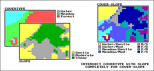 |
| Figure 2. Point-by point overlaying operations summarize the location specific coincidence of two or more maps. In this example, each map location is assigned a unique value identifying the COVERTYPE and SLOPE conditions at that location. |
Functions that relate to simple statistical parameters such as maximum, minimum, median, mode, majority, standard deviation or weighted average may also be applied in this manner. The type of data being manipulated dictates the appropriateness of the mathematical or statistical procedure used. For example, the addition of qualitative maps such as soils and land use would result in mathematically meaningless sums, since their thematic values have no numerical relationship. Other map overlay techniques include several that might be used to process either quantitative or qualitative data and generate values which can likewise take either form. Among these are masking, comparison, calculation of diversity, and permutations of map categories (as depicted in Figure 2).
More complex statistical techniques may also be applied in this manner, assuming that the inherent interdependence among spatial observations can be taken into account. This approach treats each map as a variable, each point as a case, and each value as an observation. A predictive statistical model can then be evaluated for each location, resulting in a spatially continuous surface of predicted values. The mapped predictions contain additional information over traditional non-spatial procedures, such as direct consideration of coincidence among regression variables and the ability to spatially locate areas of a given level of prediction.
An entirely different approach to overlaying maps involves category-wide summarization of values. Rather than combining information on a point-by-point basis, this group summarizes the spatial coincidence of entire categories shown on one map with the values contained on another map(s). Figure 3 contains an example of a category-wide overlay operation using the same input maps as those in Figure 2. In this example, the categories of the COVER type map are used to define an area over which the coincidental values of the SLOPE map are averaged. The computed values of average slope are then assigned to each of the cover type categories.
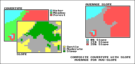 |
| Figure 3. Category-wide overlay operations summarize the spatial coincidence of map categories. In this example, each of the three COVERTYPES (open water, meadow and forest) is assigned a value equal to the average of the SLOPE values occurring within its boundaries. |
Summary statistics which can be used in this way include the total, average, maximum, minimum, median, mode, or minority value; the standard deviation, variance, or diversity of values; and the correlation, deviation, or uniqueness of particular value combinations. For example, a map indicating the proportion of undeveloped land within each of several counties could be generated by superimposing a map of county boundaries on a map of land use and computing the ratio of undeveloped land to the total land area for each county. Or a map of zip code boundaries could be superimposed over maps of demographic data to determine the average income, average age, and dominant ethnic group within each zip code.
As with location-specific overlay techniques, data types must be consistent with the summary procedure used. Also of concern is the order of data processing. Operations such as addition and multiplication are independent of the order of processing. Other operations, such as subtraction and division, however, yield different results depending on the order in which a group of numbers is processed. This latter type of operations, termed non-commutative, cannot be used for category-wide summaries.
MEASURING DISTANCE AND CONNECTIVITY
Most geographic information systems contain analytic capabilities for reclassifying and overlaying maps. These operations address the majority of applications that parallel manual map analysis techniques. However, to more fully integrate spatial considerations into decision-making, new techniques are emerging. The concept of distance has been historically associated with the "shortest straight-line distance between two points." While this measure is both easily conceptualized and implemented with a ruler, it is frequently insufficient in an environmental modeling context. A straight-line route may indicate the distance "as the crow flies," but offer little information for a walking or hitch-hiking crow, or other flightless creature. Equally important to most travelers is to have the measurement of distance expressed in more relevant terms, such as time or cost. "Rubber rulers" best characterizes the group of operations concerned with measuring effective distance.
Any system for the measurement of distance requires two components— a standard measurement unit and a measurement procedure. The measurement unit used in most computer-oriented systems is the "grid space" implied by the superimposing of an imaginary grid over a geographic area. A ruler with its uniform markings implies such a grid each time it is laid on a map. The measurement procedure for determining actual distance from any location to another involves counting the number of intervening grid spaces and multiplying by the map scale. If the grid pattern is fixed, the length of the hypotenuse of a right triangle formed by the grid is computed.
This concept of point-to-point distance may be expanded to one of proximity. Rather than sequentially computing the distance between pairs of locations, concentric equidistant zones are established around a location, or set of locations. This is analogous to the wave pattern generated when a rock is thrown into a still pond. Insert (a) in Figure 7 is an example of a simple proximity map indicating the shortest, straight-line distance from the Ranch to all other locations. A more complex proximity map would be generated if, for example, all housing locations were considered target locations-- in effect, throwing a handful of rocks. The result would be a map of proximity indicating the shortest straight-line distance to the nearest target area (i.e., house) for each non-target location.
Within many application contexts, however, the shortest route between two locations may not always be a straight line, and even if it is straight, the Euclidean length of that line may not always reflect a meaningful measure of distance. Rather, distance in these applications is best defined in terms of movement expressed as travel-time, cost, or energy that may be consumed at rates which vary over time and space. Distance- modifying effects may be expressed cartographically as "barriers" located within the space in which the distance is being measured. This implies that distance is the result of some sort of movement over that space and through those barriers.
Two major types of barriers can be identified as to how they affect the implied movement. Absolute barriers are those which completely restrict movement, and, therefore, imply an infinite distance between the points they separate, unless a path around the barrier is available. A river might be regarded as an absolute barrier to a non-swimmer. To a swimmer or a boater, however, the same river might be regarded as a relative rather than an absolute barrier. Relative barriers are ones that are passable, but only at a cost that might be equated with an increase in physical distance.
Insert (b) of Figure 4 shows a map of hiking time around the target location identified by the ranch. The map was generated by reclassifying the various cover/slope categories (see Figure 2) in terms of their relative ease of foot-travel. In the example, two types of barriers are used. The lake is treated as an absolute barrier, completely restricting hiking. The land areas, on the other hand, represent relative barriers that indicate varied hiking impedance of each point as a function of the cover/slope conditions occurring at that location.
In a similar manner, movement by automobile may be effectively constrained to a network of roads (absolute barriers) of varying speed limits (relative barriers) to generate a riding travel-time map. Or, from an even less conventional perspective, weighted distance can be expressed in such terms as the accumulated cost of powerline construction from an existing trunkline to all other locations in a study area. The cost surface that is developed can be a function of a variety of social and engineering factors, such as visual exposure and adverse topography, expressed as absolute and/or relative barriers.
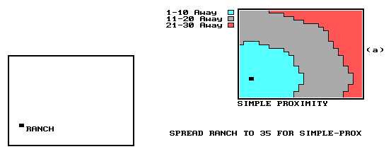 |
Figure 4. Distance between locations can be determined as simple distance or a function of the effect of absolute and relative barriers. In this example, inset (a) identifies equidistance zones around the RANCH. |
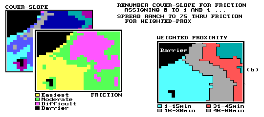 |
Inset (b) is a map of hiking travel-time from the RANCH. It was generated by considering the relative ease of travel through various COVER and SLOPE conditions (see Figure 3) where flat meadows are the fastest to traverse, steep forested are intermediate and flat water is an absolute barrier to hiking. |
The ability to move, whether physically or abstractly, may vary as a function of the implied movement as well as the static conditions at a location. Direction is one aspect of movement that can affect the ability of a barrier to restrict that movement. A topographic incline, for example, will generally impede hikers differently depending on whether their movement is uphill, downhill, or across slope. Another possible modifying factor is accumulation. After hiking a certain distance, "molehills" tend to become disheartening "mountains," and movement is more restricted.
Momentum and speed are forms of a third attribute of movement that might dynamically alter the effect of a barrier. If an old car is stopped on a steep hill, it may not be able resume movement, whereas if it were allowed to maintain its momentum (i.e., green traffic light), it could easily reach the top. Similarly, a highway impairment that effectively reduces traffic speeds from 55 to 40 miles per hour, for example, would have little or no effect during rush hour when traffic is already moving at a much slower speed.
Another distance-related class of operations is concerned with the nature of connectivity among locations on an overlay. Fundamental to understanding these procedures is the conceptualization of an accumulation surface. If the thematic value of a simple proximity map from a point is used to indicate the third dimension of a surface, a uniform bowl would be formed. The surface configuration for a weighted proximity map would have a similar appearance; however, the bowl would be warped with numerous ridges and pinnacles. Also, the nature of the surface is such that it cannot contain saddle points (i.e., false bottoms). This "bowl-like" topology is characteristic of all accumulation surfaces and can be conceptualized as a football stadium with each successive ring of seats identifying concentric, equidistant halos.
The bowl need not be symmetrical, however, and may form a warped surface responding to varying rates of accumulation. The three-dimensional insert (a) in Figure 5 shows the surface configuration of the hiking travel time map from the previous Figure 4. The accumulated distance surface is shown as a perspective plot in which the ranch is the lowest location and all other locations are assigned progressively larger values of the shortest distance, but not necessarily straight, to the ranch. When viewed in perspective, this surface resembles a topographic surface with familiar valleys and hills. However, in this case the highlands indicate areas that are effectively farther away from the ranch.
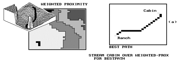 |
Figure 5. Connectivity operations characterize the nature of spatial linkages among locations. Insert (a) delineates the shortest (i.e. the least time) hiking route between the CABIN and the RANCH. The route traces the steepest downhill path along the travel-time surface derived in Figure 4 (also shown as a three-dimensional plot). |
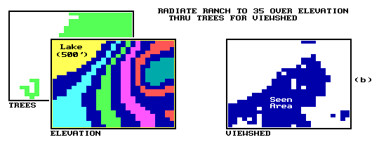 |
Inset (b) identifies the viewshed of the RANCH. The ELEVATION surface and TREES act as absolute barriers when establishing visual connectivity. |
In the case of simple distance, the delineation of paths, or connectivity, locates the shortest straight-line between two points considering only two dimensions. Another technique traces the steepest downhill path from a location over a complex three-dimensional surface. The steepest downhill path along a topographic surface will indicate the route of surface runoff. For a surface represented by a travel-time map, this technique traces the optimal (e.g., the shortest or quickest) route. Insert (a) of Figure 5 indicates the optimal hiking path from a nearby cabin to the ranch, as the steepest downhill path over the accumulated hiking-time surface shown in the previous figure.
If an accumulation cost surface is considered, such as the cost surface for power line construction described above, the minimum cost route will be located. If power line construction to a set of dispersed locations were simultaneously considered, an "optimal path density" map could be generated which identifies the number of individual optimal paths passing through each location from the dispersed termini to the trunk line. Such a map would be valuable in locating major feeder lines (i.e., areas of high optimal path density) radiating from the central trunk line.
Another connectivity operation determines the narrowness of features. The narrowness at each point within a map feature is defined as the length of the shortest line segment (i.e., chord) which can be constructed through that point to diametrically opposing edges of the feature. The result of this processing is a continuous map of features with lower values indicating relatively narrow locations. For a narrowness map of forest stands, low thematic values indicate interior locations with easy access to edges.
Viewshed characterization involves establishing intervisibility among locations. Locations forming the viewshed of an area are connected by straight rays in three-dimensional space to the "viewer" location, or a set of viewers. Topographic relief and surface objects form absolute barriers that preclude connectivity. If multiple viewers are designated, locations within the viewshed may be assigned a value indicating the number or density of visual connections. Insert (b) of Figure 8 shows a map of the viewshed of the ranch, considering the terrain and forest canopy height as visual barriers.
CHARACTERIZING NEIGHBORHOODS
The fourth and final group of operations includes procedures that create a new map where the value assigned to a location is computed as a function of independent values surrounding that location (i.e., its cartographic neighborhood). This general class of operations can be conceptualized as "roving windows" moving throughout the mapped area. The summary of information within these windows can be based on the configuration of the surface (e.g., slope and aspect) or the mathematical summary of thematic values.
The initial step in neighborhood characterization is the establishment of neighborhood membership. The members are uniquely defined for each target location as the set of points which lie within a specified distance and direction around that location. In most applications, the window has a uniform geometric shape and orientation (e.g., a circle or square). However, as noted in the previous section, the distance may not necessarily be Euclidean nor symmetrical, such as a neighborhood of "down-wind" locations within a quarter mile of a smelting plant. Similarly, a neighborhood of "the ten-minute drive" along a road network could be defined.
The summary of information within a neighborhood may be based on the relative spatial configuration of values that occur within the window. This is true of the operations which measure topographic characteristics, such as slope, aspect, or profile from elevation values. One such technique involves the "least squares fit" of a plane to adjacent elevation values. This process is similar to fitting a linear regression line to a series of points expressed in two- dimensional space. The inclination of the plane denotes terrain slope and its orientation characterizes the aspect. The window is successively shifted over the entire elevation map to produce a continuous slope or a continuous aspect map. Insert (a) of Figure 6 shows the derived map of aspect for the area.
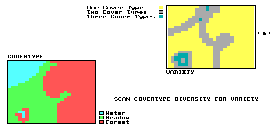 |
Figure 9. Neighborhood operations summarize the attributes occurring in the vicinity of each location. Inset (a) is a map of COVERTYPE diversity generated by counting the number of different COVERTYPES in the immediate vicinity of each map location. |
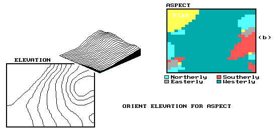 |
Inset (b) is a map of topographic aspect generated by successively fitting a plane to neighborhoods of adjoining ELEVATION values. |
Note that a slope map of any surface represents the first derivative of that surface. For an elevation surface, slope depicts the rate of change in elevation. For an accumulation cost surface, its slope map represents the rate of change in cost (i.e., a map of marginal cost). For a travel-time overlay, its slope map indicates relative change in speed and its aspect map identifies direction of travel at each location. Also, the slope map of an existing topographic slope map (i.e., second derivative) will characterize surface roughness.
The creation of a profile map uses a window defined as the three adjoining points along a straight line oriented in a particular direction. Each set of three values can be regarded as defining a cross-sectional profile of a small portion of a surface. Each line of data is successively evaluated for the set of windows along that line. This procedure may be conceptualized as slicing a loaf of bread, then removing each slice and characterizing its profile (as viewed from the side) in small segments along its upper edge. The center point of each three-member neighborhood is assigned a value indicating the profile form at that location. The value assigned can identify a fundamental profile class (e.g., inverted "V' shape indicates a ridge or peak) or it can identify the magnitude, in degrees, of the "skyward angle" formed by the intersection of the two line segments of the profile.
The result of this operation is a continuous map of a surface's profile as viewed from a specified direction. Depending on the resolution of an elevation map, its profile map could be used to identify gullies or valleys running east/west (i.e, "V" shape as viewed from the east or west profile) or depressions (i.e., "V" shape as viewed from both the east and west).
The other group of neighborhood operations are those that summarize thematic values. Among the simplest of these is the calculation of summary statistics associated with the map categories occurring within each neighborhood. These statistics might include, for example, the maximum income level, the minimum land value, or the diversity of vegetation types within an eighth-mile radius (or perhaps, a five-minute walking radius) of each target point. Insert (b) of Figure 6 shows the cover type diversity occurring within the immediate vicinity of each map location. Other thematic summaries might include the total, the average, or the median value occurring within each neighborhood; the standard deviation or variance of those values; or the difference between the value occurring at a target point itself and the average of those surrounding it.
Note that none of the neighborhood characteristics described so far relate to the amount of area occupied by the map categories within each neighborhood. Similar techniques might be applied, however, to characterize neighborhood values which are weighted according to areal extent. One might compute, for example, total land value within three miles of each target point on a per-acre basis. The consideration of the size of the neighborhood components also gives rise to several additional neighborhood statistics including mode (i.e., the value associated with the greatest proportion of neighborhood areas, minority value (i.e., the value associated with the smallest proportion of a neighborhood area), and uniqueness (i.e., the proportion of the neighborhood area associated with the value occurring at the target point itself).
Another location attribute which might be used to modify thematic summaries is the cartographic distance from the target point. While distance has already been described as the basis for defining a neighborhood's absolute limits, it might also be used to define the relative weights of values within the neighborhood. Noise level, for example, might be measured according to the inverse square of the distance from surrounding sources.
The azimuthal relationship between neighborhood location and the target point may also be used to weight the value associated with that location. In conjunction with distance weighting, this gives rise to a variety of spatial sampling and interpolation techniques. For example, "weighted nearest-neighbors" interpolation of lake bottom temperature data assigns a value to an unsampled location as the distance-weighted average temperature of a set of sampled points within its vicinity.
GENERALIZED GIS MODELING APPROACH
As an example of some of the ways in which fundamental map processing operations might be combined to perform more complex analyses, consider the cartographic model outlined in Figure 7. Note the format uses boxes to represent encoded and derived maps and lines to represent primitive map processing operations. The flowchart structure indicates the logical sequencing of operations on the mapped data that progresses to the desired final map.
The simplified cartographic model shown depicts the siting of the optimal corridor for a highway considering only two criteria: an engineering concern to avoid steep slopes and a social concern to avoid visual exposure. Implementation of the model using the pMAP system requires less than 25 lines of code. The execution of the entire model using the data base in the previous figures requires less than three minutes in a 386SX notebook personal computer that fits in a briefcase. Such processing power was the domain of a mainframe computer just a decade ago, which effectively made GIS technology out of reach for most users.
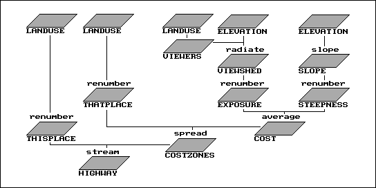 |
| Figure 7. This simplified cartographic model depicts the siting of an optimal corridor for a highway with reference to only two criteria: an engineering concern to avoid steep slopes and a social concern to avoid visual exposure. In a manner similar to conventional algebra, this process uses a series of map operations (indicated by lines) to derive intermediate maps (indicated by boxes), leading to a final map of the optimal corridor. |
Given a map of topographic elevation values and a map of land use, the model allocates a minimum-cost highway alignment between two predetermined termini. Cost is not measured in dollars, but in terms of location criteria. The right portion of the flowchart develops a "discrete cost surface" in which each location is assigned a relative cost based on the particular steepness/ exposure combination occurring at that location. For example, those areas that are flat and not visible from houses would be assigned low values (good places for a road); whereas areas on steep slopes and visually exposed would be assigned high values (bad places for a road).
Similar to the hiking example described in Figures 4 and 5, the discrete cost surface is used as a map of relative barriers for establishing an "accumulated cost surface" from one of the termini to all other locations within the mapped area. The final step locates the other terminus on the accumulated cost surface and identifies the minimum cost route as the steepest downhill path along the surface from that point to the bottom (i.e., the other end point).
In addition to the benefits of efficient data management and of automating cartographic procedures, the modeling structure of computer-assisted map analysis has several other advantages. Foremost among these is the capability of dynamic simulation (i.e., spatial "what if" analysis). For example, the highway siting model could be executed for several different relative weightings of the engineering and social criteria. What if the terrain steepness is more important? Or what if the visual exposure is twice as important? Where does the minimum cost route change, or just as important, where does it not change? From this perspective, the model "replies" to user inquires, rather than an "answering" them-- providing information, rather than tacit decisions.
Another advantage to cartographic modeling is its flexibility. New considerations may be easily added and existing ones refined. For example, the non-avoidance of open water bodies in the highway model is a major engineering oversight. In its current form, the model favors construction on lakes, as they are flat and frequently not visually exposed. This new requirement can be readily incorporated by identifying open water bodies as absolute barriers (i.e., infinite cost) when constructing the accumulation cost surface. The result will be routing of the minimal cost path around these areas of extreme cost.
Finally, cartographic modeling provides an effective structure for communicating both specific application considerations and fundamental processing procedures. The flowchart structure provides a succinct format for communicating the logic, assumptions, and relationships embodied in an analysis. Such a presentation encourages decision-makers' active involvement in the analytic process.
CARTOGRAPHIC VERSUS SPATIAL MODELING
Resource and environmental modeling are pushing at the frontier of GIS technology. To the user, a model is an abstraction of reality used to gain conceptual clarity and improve understanding of a system. GIS, by its inherent nature, is an abstraction of landscape complexity. The merging of these modeling and GIS technology is inevitable, but the form of the merger is not yet clear.
The cartographic model of the land planner described in the previous section is different from many modelers' concept of a model. It is basically an implementation of procedures that would be used in a manual map analysis. In this sense, the model serves as a "recipe" for siting alternative highway corridors. It is the subjective expression of map variables responding to various weighting factors. It is a non-process model with minimal mathematical rigor, in which the GIS acts as a conceptual blackboard for decision-making.
Contrast this type of model with one determining the surface water flow over the landscape. In this application, extensive mathematical equations have been developed to describe the physical process and closely track the cause and effect of a system. It is a process model whose empirical relationships are rigorously expressed in mathematical terms.
For the process-oriented modeler, the mathematical relationships are usually parameterized with spatially aggregated values, such as the average slope and dominant soil of an entire watershed. A generalized model assumes "if it is steep over here, but flat over there, then it must be moderately sloped everywhere," as it uses the average slope in the execution of a hydrologic model. From this perspective, maps are used to generalize equation parameters using traditional drafting aids, such as dot grids, planimeters and light-table overlays. Based on such experiences with maps, the modeler initially views GIS as an automated means of deriving model parameters that are passed as input to existing models.
An alternative perspective is the spatial model, and its implied 'map-ematics.' In this context, the GIS provides not only the definition of model parameters, but the engine of the model itself. The result is a full integration of GIS and a mathematical model. A major advantage of this approach is that input variables are defined as continuous surfaces, and areas different from the 'average' can recognized in the model. Another advantage is that spatially dependent operators, such as effective distance, can be incorporated. A third advantage is the ability to deal with error propagation in models.
The 1960's and 70's saw the development of computer mapping and spatial data base management. The extension of these fields to a robust set of analytical capabilities and cartographic modeling applications became the focus of the 1980's. Spatial modeling is a direct extension of cartographic modeling and will likely dominate future research. The two modeling approaches can be seen as the extremes of a continuum in the mathematical rigor used in modeling applications.
To move toward spatial modeling and the full implementation of "map-ematics," several conditions must be met. On one front, the GIS community must become familiar with the process modeler's requirements and incorporate the more mathematical functionality into their GIS products. On the other front, the modeling community must see GIS as more than an electronic planimeter and become familiar with the conditions, considerations and analytical capabilities of the technology. This dialogue between modelers and GIS specialists has begun in earnest and will focal point for GIS research.
SUMMARY AND CONCLUSIONThe preceding discussion developed a topology for computer-assisted map analysis, described a set of independent analytical operations common to a broad range of applications and suggested GIS's role in environmental modeling. By systematically organizing these operations, the basis for a modeling approach is identified. This approach accommodates a variety of analytic procedures in a common, flexible and intuitive manner, analogous to the mathematical structure of conventional algebra.
Environmental modeling has always required spatial information as its cornerstone. However, procedures for fully integrating this information into the modeling process have been limited. Traditional statistical approaches seek to constrain the spatial variability within the data. Sampling designs involving geographic stratification attempt to reduce the complexity of spatial data. However, it is the spatially induced variation of mapped data and their interactions that most often concern environmental modelers. This approach retains the quantitative aspects of the data necessary for most models, but lacks spatial continuity. On the other hand, the drafting approach is spatially precise, but limited by both its non-quantitative nature and laborious procedures. In most instances, a final drafted map represents an implicit decision considering only a few possibilities, rather than a comprehensive presentation of information.
Computer-assisted map analysis, on the other hand, involves quantitative expression of spatially consistent data. In one sense, this technology is similar to conventional map processing involving traditional maps and drafting aids, such as pens, rub-on shading, rulers, planimeters, dot grids and acetate sheets for light-table overlays. In another sense, these systems provide advanced analytic capabilities, enabling modelers to address complex systems in entirely new ways. Within this analytic context, mapped data truly becomes spatial information for inclusion in environmental models. The GIS itself becomes an integral part of the model by providing both the mapped variables and the processing environment.
________________________________
REFERENCES
Berry, J.K., 1996. "GIS Modeling: A Conceptual Framework and Its Practical Expression," book chapter in GIS Applications in Natural Resources 2, GIS World Books, Fort Collins, Colorado, pp. 123-134.
Berry, J.K., 1993. "Cartographic Modeling: The Analytic Capabilities of GIS," book chapter in Geographic Information Systems and Environmental Modeling, Oxford University Press, Oxford, England, pp. 58-74.
Berry, J.K, 1987a. "Fundamental Operations in Computer-assisted Map Analysis," book chapter in Fundamentals of Geographic Information Systems: A Compendium, ASPRS, Falls Church, Virginia, pp. 206-211.
Berry, J.K. 1987b. "Fundamental Operations in Computer-assisted Map Analysis," International Journal of Geographical Information Systems, Vol. 1, No. 2, pp. 119-136.
Berry, J.K., 1986a. "Learning Computer-Assisted Map Analysis," Journal of Forestry, October, 1986, pp. 39-43.
Berry, J.K., 1986b. "A Mathematical Structure for Analyzing Maps," Environmental Management, Vol 11(3): 317-325.