Topic 5 Exercises
Access MapCalc using the Tutor25.rgs
by selecting Startà Programsà MapCalc
Learnerà MapCalc Learnerà Open existing
map setà MapCalc Dataà Tutor25.rgs. The following set of exercises utilizes this
database.
5.1 Calculating Viewsheds
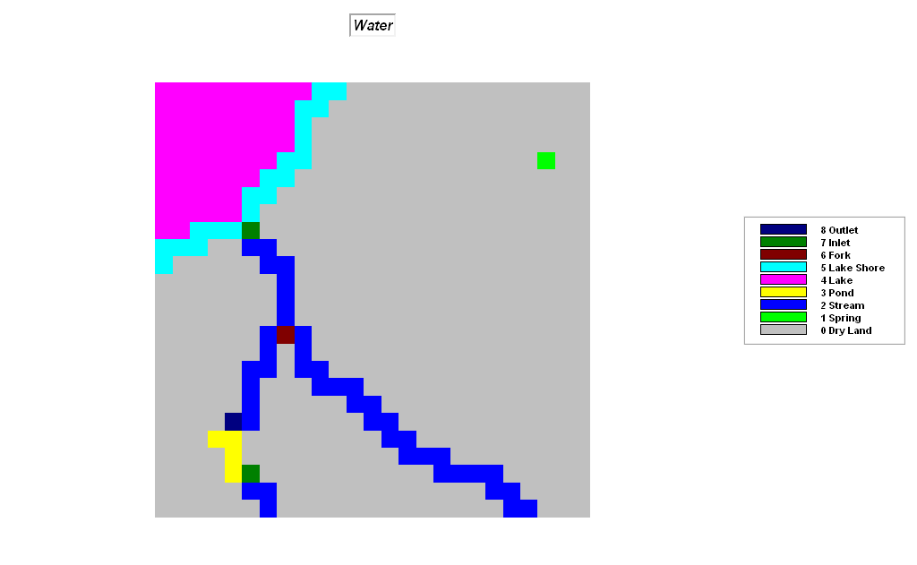
 Use the View
button (binocular icon) to select and display the Water map.
Use the View
button (binocular icon) to select and display the Water map.
Note that there are eight
different types of water depending on its flow.

 Press the Map
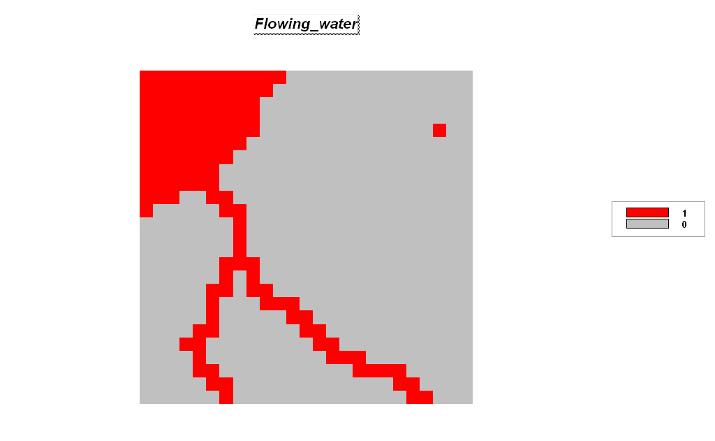
Analysis button and choose Reclassifyà Renumber
to access the dialog box for reclassifying map values. Complete the input specifications as shown
below to derive a binary map of Flowing
Water
Press the Map
Analysis button and choose Reclassifyà Renumber
to access the dialog box for reclassifying map values. Complete the input specifications as shown
below to derive a binary map of Flowing
Water
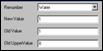
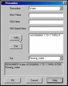
 Select the Water map from the drop-down list, then specify 1 as the NewValue, 1 as the OldValue and 8 as the OldUpperValue. Press the Add button to submit the reassignment phrase. Specify Flowing_water
as the new map name and press OK to
create a binary map where 1= any water type and 0 = not water.
Select the Water map from the drop-down list, then specify 1 as the NewValue, 1 as the OldValue and 8 as the OldUpperValue. Press the Add button to submit the reassignment phrase. Specify Flowing_water
as the new map name and press OK to
create a binary map where 1= any water type and 0 = not water.
 RENUMBER Water ASSIGNING 1 TO 1 THRU 8 FOR Flowing_water
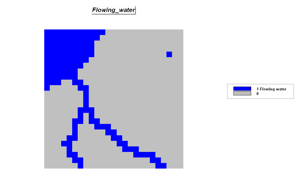
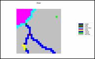
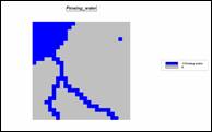
 Press the Use Cells button to set the display type to Grid.
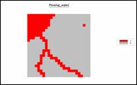

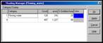
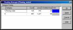 Press the Shading Manager button then enter “Flowing water” as the category description. Double-click on the red Color and choose blue
from the color pallet. Click OK to submit the display changes.
Press the Shading Manager button then enter “Flowing water” as the category description. Double-click on the red Color and choose blue
from the color pallet. Click OK to submit the display changes.

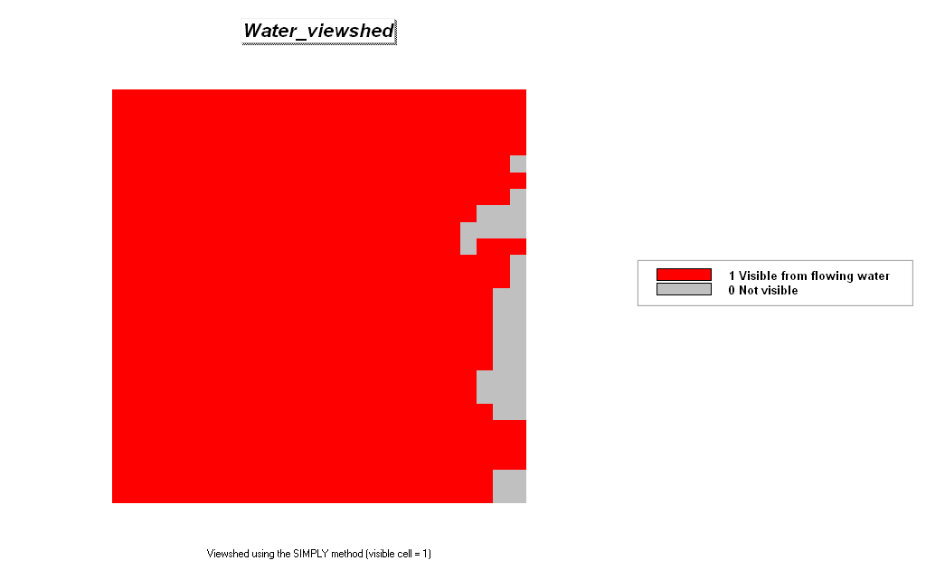
 Press the Map Analysis button and choose Distanceà Radiate to
access the dialog box for visual analysis.
Complete the input specifications as described below to derive a binary
map of Water_viewshed.
Press the Map Analysis button and choose Distanceà Radiate to
access the dialog box for visual analysis.
Complete the input specifications as described below to derive a binary
map of Water_viewshed.
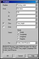
 Press the Help button to get a description of the Radiate command’s function and input fields. Specify…
Flowing_water
as the viewersMap
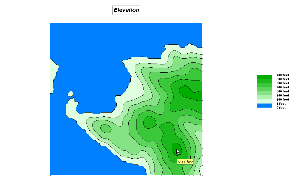
Elevation as
the surfaceMap
100 as the # of grid spaces away
1 as the viewer_heightValue
Simply as the
calculation mode (binary viewshed)
Water_viewshed
as the newMap
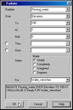 RADIATE Flowing_water OVER Elevation TO 100 AT 1 NULLVALUE 0
Simply FOR Water_viewshed
RADIATE Flowing_water OVER Elevation TO 100 AT 1 NULLVALUE 0
Simply FOR Water_viewshed

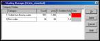 Double-click on the map legend to pop-up the Shading Manager dialog box. Enter a description for the map Categories as 1= “Visible from flowing
water” and 0= “Not visible.” Note that
approximately 95% of the project area is visually connected to flowing water
and that the few “Not visible” areas are concentrated along the eastern edge.
Double-click on the map legend to pop-up the Shading Manager dialog box. Enter a description for the map Categories as 1= “Visible from flowing
water” and 0= “Not visible.” Note that
approximately 95% of the project area is visually connected to flowing water
and that the few “Not visible” areas are concentrated along the eastern edge.
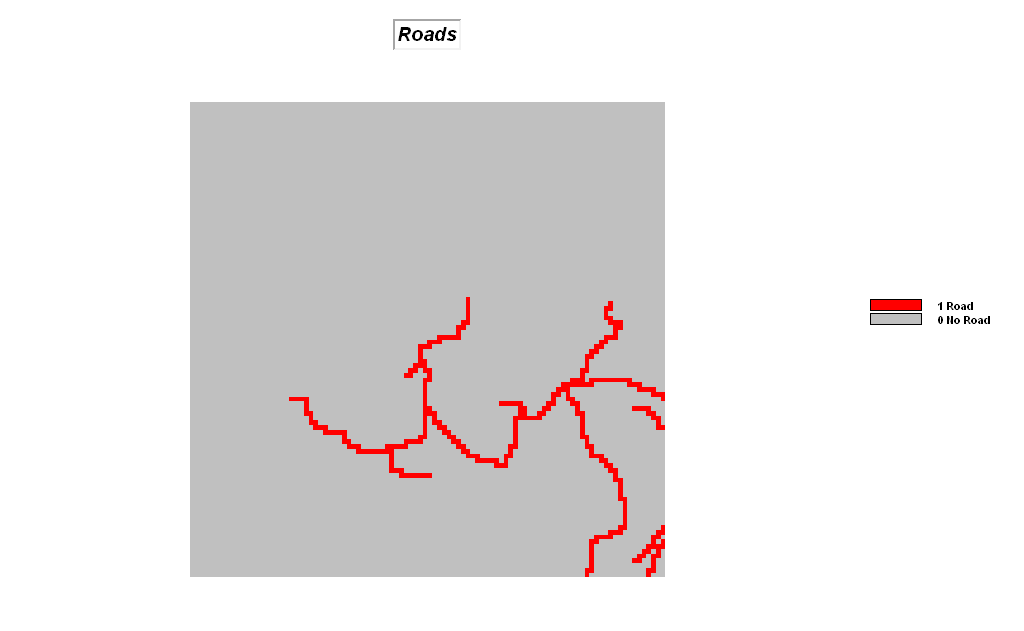
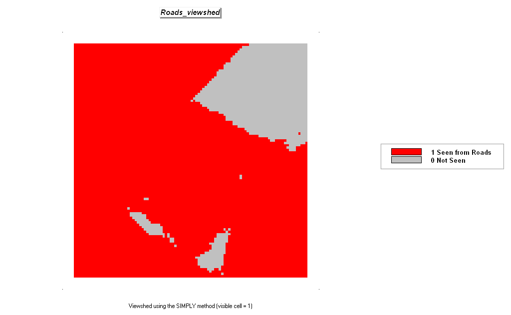
On your own, follow a similar
visual analysis procedure to generate a viewshed
map (Roads_viewshed) of any road
location (based on the Roads_type
map). What percent of the project area
is visually connected to roads?
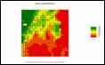
5.2 Calculating Visual Exposure
 Press the Map Analysis button and choose Distanceà Radiate to
access the dialog box for visual analysis.
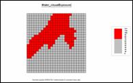
Complete the input specifications as shown below to derive a visual
exposure map showing “how many” water grid cells are visually connected to
every location within in the project area.
Press the Map Analysis button and choose Distanceà Radiate to
access the dialog box for visual analysis.
Complete the input specifications as shown below to derive a visual
exposure map showing “how many” water grid cells are visually connected to
every location within in the project area.
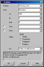 RADIATE Flowing_water OVER Elevation TO 100 AT 1 NULLVALUE 0
Completely FOR Water_visualExposure
RADIATE Flowing_water OVER Elevation TO 100 AT 1 NULLVALUE 0
Completely FOR Water_visualExposure
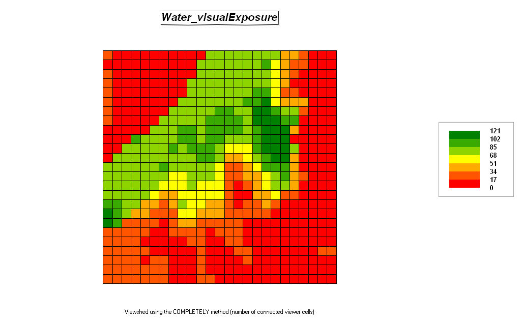
Selecting the “Completely” calculation mode identifies
the number of connected viewer cells. Larger
values indicate higher visual exposure to water—locations that “seen” from a
lot of water locations (and by direct line-of-sight, “see” a lot from water
locations).
 Press the Layer Mesh button to superimpose the analysis grid. Press the Use Cells button to set the display type to Grid.
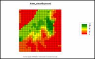
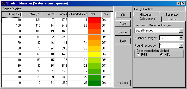
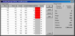
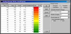
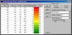
 Double-click on the legend to pop-up the Shading Manager. Change the Number of ranges to 12. Note that the data intervals are expressed as
increasing steps of 10 additional viewer cells (water locations).
Double-click on the legend to pop-up the Shading Manager. Change the Number of ranges to 12. Note that the data intervals are expressed as
increasing steps of 10 additional viewer cells (water locations).
Under the Lock column, click Off the automatically assigned yellow
inflection point for the range 30 to 40.
Click the Color block for
range for 50 to 60 and select yellow
from the pallet to reset the color inflection point on the color ramp. Switch the colors for the minimum and maximum
ranges by clicking on the respective color blocks and choose green for the lowest range and red for the highest range. Press OK
to generate the new display.

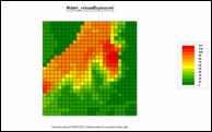
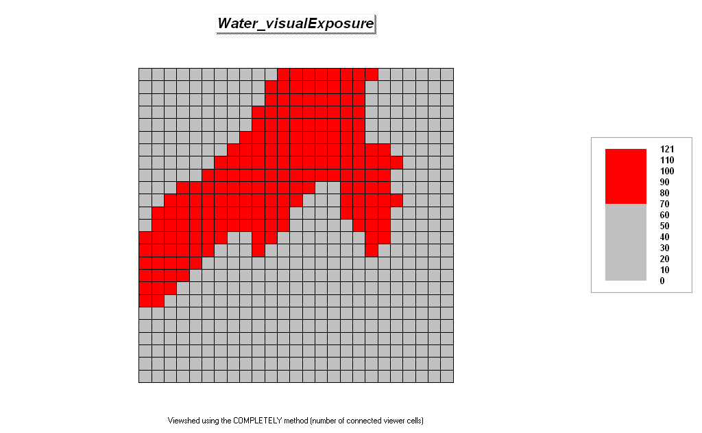
Use the Shading Manager to create a display that isolates the areas of very
high visual exposure (70 or more water locations visible) as red with a background
of grey—set grey as the Color from 0-10 through the 60-70
intervals and Lock on red for the 70-80 and 110-121ranges.
On your own, follow a similar
visual analysis procedure to generate a visual
exposure map (Roads_visualExposure)
of any road location (based on the Roads_type
map). What is the highest visual
exposure to roads in the project area?
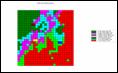
5.3 Accounting for Screens
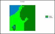
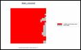
Use the View
button (binocular icon) to select and display the Covertype map.
 Use the Map
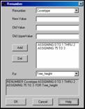
Analysis button and choose Reclassifyà Renumber to access its dialog box and complete as shown.
Use the Map
Analysis button and choose Reclassifyà Renumber to access its dialog box and complete as shown.
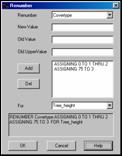 RENUMBER Covertype ASSIGNING 0 TO 1 THRU 2 ASSIGNING 75 TO 3 FOR Tree_height
Do not forget to press the
Add button to enter each Renumber
phrase…
ASSIGNING 0 TO 1 THRU 2
(Water & Meadow)
ASSIGING 75 TO 3 (Forest)
…to indicate the height of
the vegetation canopy (same units as the Elevation map). This assigns 0 feet (NewValue) for Water (Oldvalue=
1) and Meadow (OldValue= 2) locations
and 75 feet (NewValue) for Forest
locations (OldValue= 3).
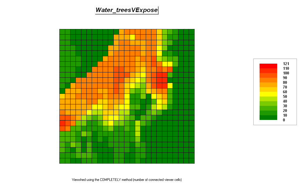
Press the Map Analysis button and choose Distanceà Radiate to
access the dialog box for visual analysis.
Complete the input specifications as described below to derive a visual
exposure map accounting for the height of the tree canopy.
 RADIATE Flowing_water OVER Elevation TO 100 AT 1 NULLVALUE 0
THRU Tree_height Completely FOR Water_treesVExpose
RADIATE Flowing_water OVER Elevation TO 100 AT 1 NULLVALUE 0
THRU Tree_height Completely FOR Water_treesVExpose
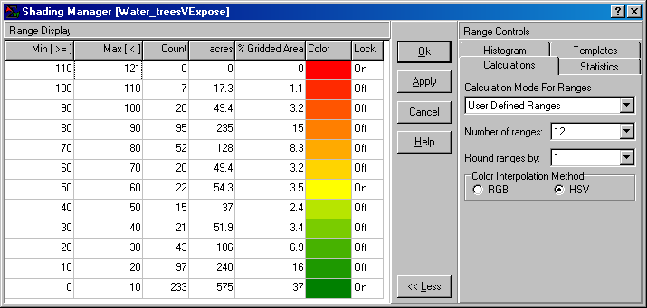
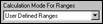
Double-click on the legend to pop-up the Shading Manager. Change the Number of ranges to 12.
 Change the Calculation Mode to User
Defined Ranges.
Change the Calculation Mode to User
Defined Ranges.
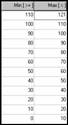
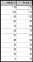 Starting at the bottom of the Min [>=] column enter values
increasing by 10 as shown above,
then ending with 121 at the top of
the Max [<] column. Set the Color settings the same as before— green for the lowest range, red for the highest range and yellow for the 50 to 60 range. Press OK
to display the map using the custom legend that is the same as used for
displaying the Water_visualExposure
map generated in the previous section.
Starting at the bottom of the Min [>=] column enter values
increasing by 10 as shown above,
then ending with 121 at the top of
the Max [<] column. Set the Color settings the same as before— green for the lowest range, red for the highest range and yellow for the 50 to 60 range. Press OK
to display the map using the custom legend that is the same as used for
displaying the Water_visualExposure
map generated in the previous section.

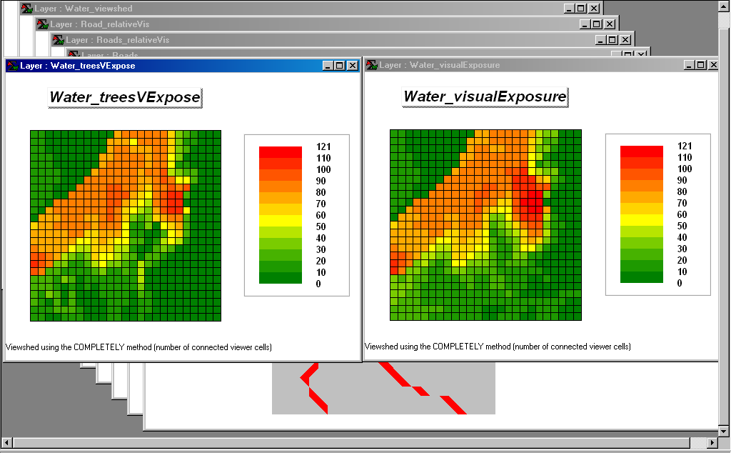
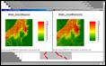
 Click on the Restore Down button in the upper-right corner of the display. Use standard Windows “click-and-drag/size”
techniques to position the Water_visualExposure
and Water_treesVExposure side by side
as shown below.
Click on the Restore Down button in the upper-right corner of the display. Use standard Windows “click-and-drag/size”
techniques to position the Water_visualExposure
and Water_treesVExposure side by side
as shown below.
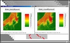
Note the visual differences
between the two maps—visual exposure with and without accounting for the height
of the tree canopy. The area of high visual
exposure (red tones) that accounts for the tree canopy barriers has a similar
shape but is smaller than the corresponding area without trees.
 Note: Each map display is contained in a separate
window. Standard Windows techniques such
as cascading, horizontal and vertical “tiling” are available.
Note: Each map display is contained in a separate
window. Standard Windows techniques such
as cascading, horizontal and vertical “tiling” are available.
5.4 Calculating Weighted Visual Exposure
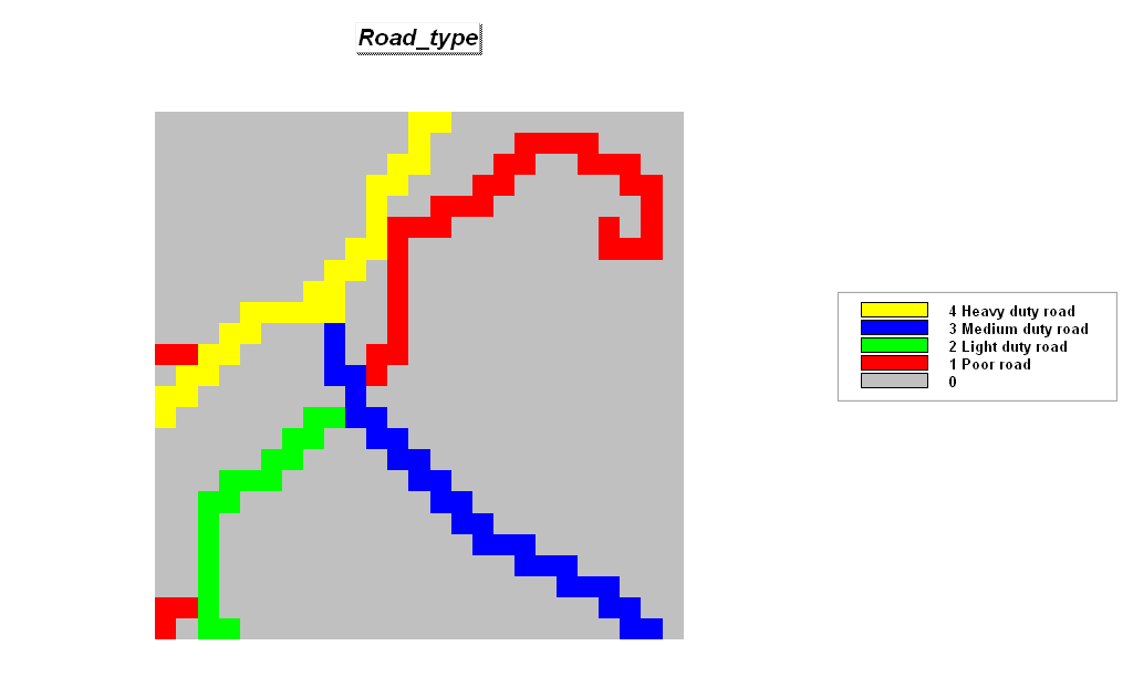
Use the View
button (binocular icon) to display the Roads_type
map.

 Press the Map
Analysis button and choose Reclassifyà Renumber
to access its dialog box and complete as shown.
Press the Map
Analysis button and choose Reclassifyà Renumber
to access its dialog box and complete as shown.
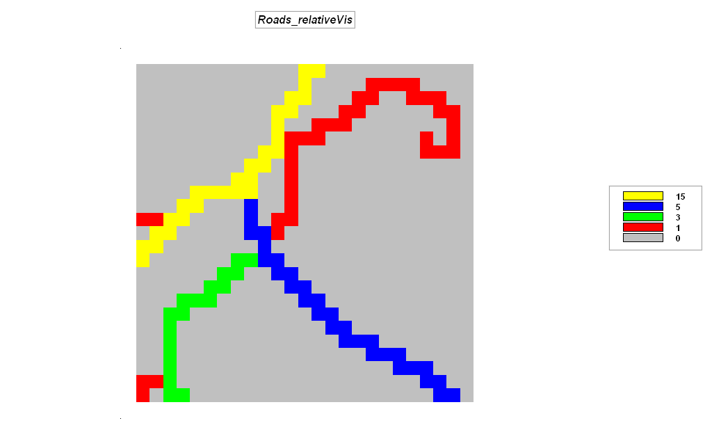
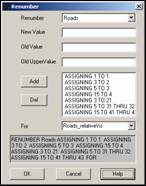 RENUMBER Roads ASSIGNING 1 TO 1 ASSIGNING 3 TO 2 ASSIGNING 5
TO 3 ASSIGNING 15 TO 4 ASSIGNING 3 TO 21 ASSIGNING 5 TO 31 THRU 32
ASSIGNING 15 TO 41 THRU 43 FOR Roads_relativeVis
RENUMBER Roads ASSIGNING 1 TO 1 ASSIGNING 3 TO 2 ASSIGNING 5
TO 3 ASSIGNING 15 TO 4 ASSIGNING 3 TO 21 ASSIGNING 5 TO 31 THRU 32
ASSIGNING 15 TO 41 THRU 43 FOR Roads_relativeVis
Do not forget to press the Add button to enter each Renumber phrase…
ASSIGNING 1 TO 1 (one
car)
ASSIGING 3 TO 2 (three
cars)
ASSIGNING 5 TO 3 (five
cars)
ASSIGNING 15 TO 4 (fifteen
cars)
…to indicate the relative
number of cars in a given period of time.

Press the Map Analysis button and choose Distanceà Radiate to
access the dialog box for visual analysis.
Complete the input specifications as shown below to derive a weighted
visual exposure map showing the relative visual exposure to roads for every
location within in the project area.
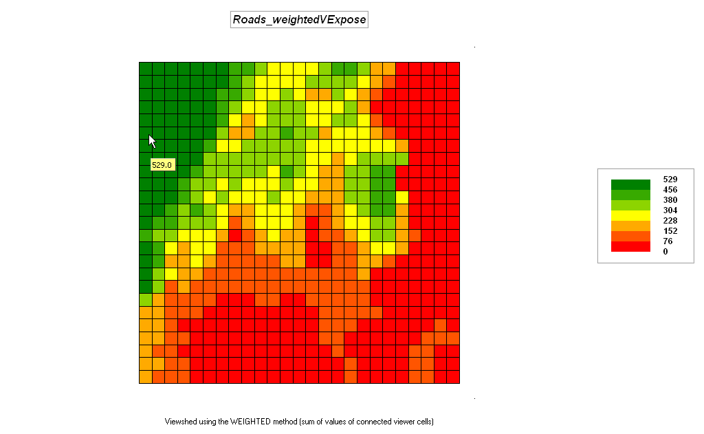
 RADIATE Road_relativeVis OVER Elevation TO 100 AT 1
NULLVALUE 0 Weighted FOR Roads_weightedVExpose
RADIATE Road_relativeVis OVER Elevation TO 100 AT 1
NULLVALUE 0 Weighted FOR Roads_weightedVExpose

 Note that the weighted visual exposure ranges
from 0 to 529. The most visually exposed
location is in the west border at column 1, row 20 as reported in the lower-left corner of the
display window as the mouse is positioned over the location on the map.
Note that the weighted visual exposure ranges
from 0 to 529. The most visually exposed
location is in the west border at column 1, row 20 as reported in the lower-left corner of the
display window as the mouse is positioned over the location on the map.
5.5 Modeling Visual Exposure Impacts
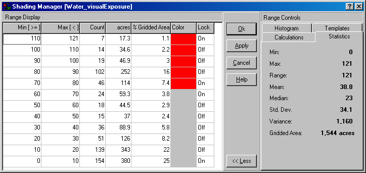
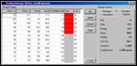
 Double-click on the Roads_weightedVExpose map’s legend to pop-up the Shading Manager. Select the Histogram tab and click Std.
Dev. button to get a plot of the data distribution. Note that the average
is about 150.
Double-click on the Roads_weightedVExpose map’s legend to pop-up the Shading Manager. Select the Histogram tab and click Std.
Dev. button to get a plot of the data distribution. Note that the average
is about 150.
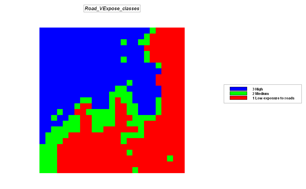
Based on the Roads_weightedVExpose data distribution,
create a map that identifies areas of…
Low= 1 (0-100 seen)
Medium= 2 (100-200 seen)
High= 3 (>200 seen)
…visual exposure by choosing Reclassifyà Renumber
and completing the dialog box as shown below.
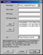 RENUMBER Roads_weightedVExpose ASSIGNING 1 TO 0 THRU
100 ASSIGNING 2 TO 100 THRU 200 ASSIGNING 3 TO 200 THRU 1000 FOR Road_VExpose_classes
RENUMBER Roads_weightedVExpose ASSIGNING 1 TO 0 THRU
100 ASSIGNING 2 TO 100 THRU 200 ASSIGNING 3 TO 200 THRU 1000 FOR Road_VExpose_classes

Notice that the area of High
visual exposure to roads is concentrated in the northwestern portion of the
project area while the areas of Low visual exposure are generally in the
southeast.
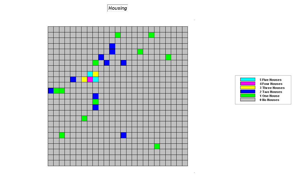
Use the View
button (binocular icon) to select and display the Housing map.

The values stored for grid
cell indicates how many houses occur at that location (1 hectare grid
cell).
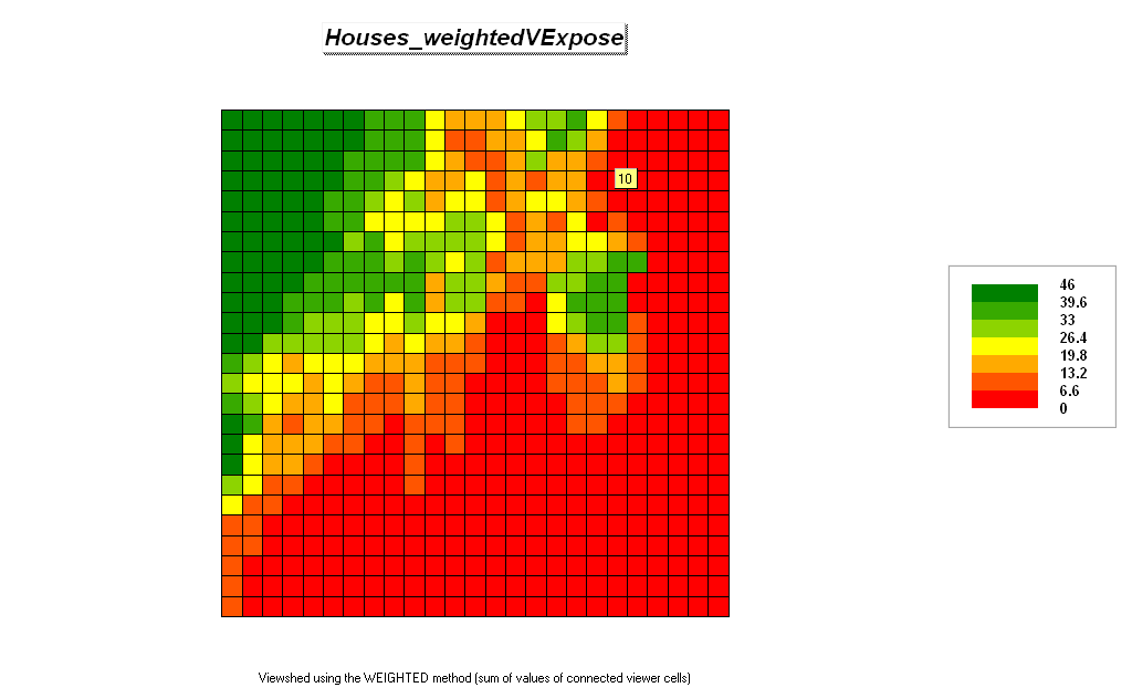
Press the Map Analysis button and choose Distanceà Radiate to
access the dialog box for visual analysis.
Complete the input specifications as shown below to derive a weighted
visual exposure map showing the relative visual exposure to houses for every
location within in the project area.
 RADIATE Housing OVER Elevation TO 100 AT 1 NULLVALUE 0
Weighted FOR Houses_weightedVExpose
RADIATE Housing OVER Elevation TO 100 AT 1 NULLVALUE 0
Weighted FOR Houses_weightedVExpose
 Use the Shading
Manager Histogram tab to get an idea
of the data distribution for the Housing_weightedVExpose
surface.
Use the Shading
Manager Histogram tab to get an idea
of the data distribution for the Housing_weightedVExpose
surface.
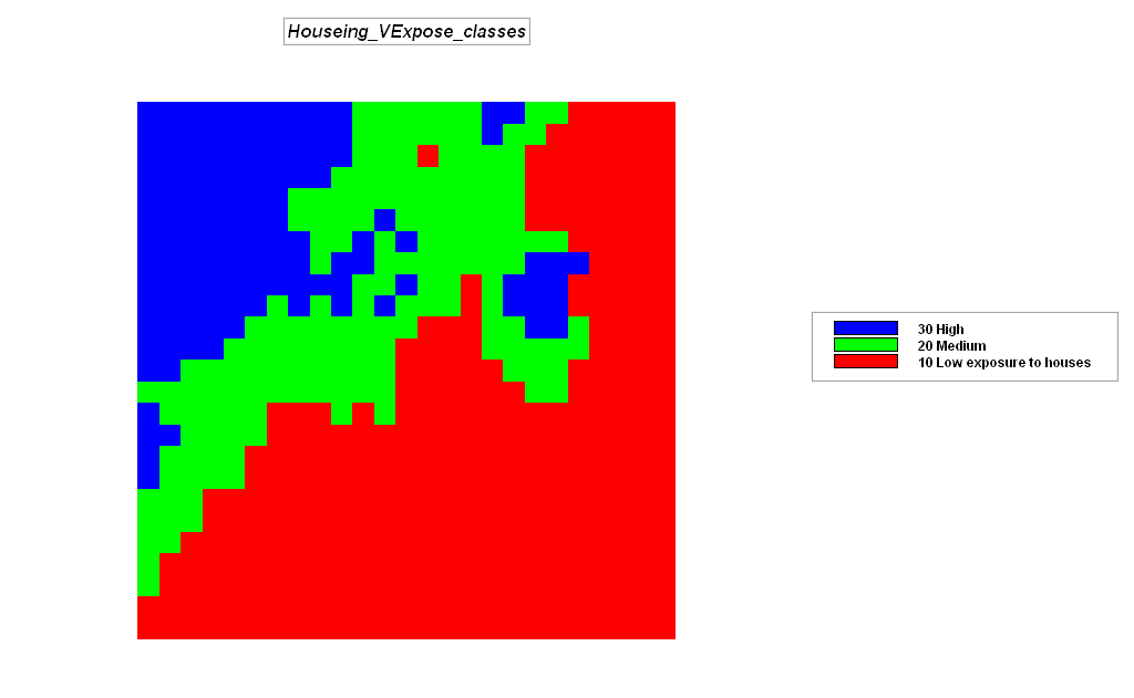
Create a map that identifies
areas of Low, Medium and High visual exposure by 1) pressing the Map Analysis button 2) choosing Reclassifyà Renumber
and 3) completing the dialog box as shown below so…
Low= 1 (0-10 houses seen)
Medium= 2 (10-30 houses seen)
High= 3 (>30 houses seen)
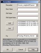 RENUMBER Houses_weightedVExpose ASSIGNING 10 TO 0 THRU 10
ASSIGNING 20 TO 10 THRU 30 ASSIGNING 30 TO 30 THRU 1000 FOR
Housing_VExpose_classes
RENUMBER Houses_weightedVExpose ASSIGNING 10 TO 0 THRU 10
ASSIGNING 20 TO 10 THRU 30 ASSIGNING 30 TO 30 THRU 1000 FOR
Housing_VExpose_classes
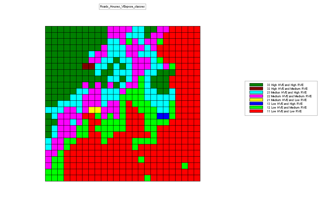
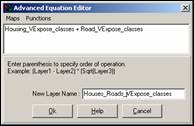
Combine the two maps
indicating the classes of visual exposure to roads and houses by Map Analysisà Overlayà Calculate
and completing the following dialog box as shown below.
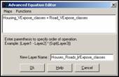 CALCULATE Housing_VExpose_classes + Road_VExpose_classes FOR
Houses_Roads_VExpose_classes
CALCULATE Housing_VExpose_classes + Road_VExpose_classes FOR
Houses_Roads_VExpose_classes
 To select a map, select Maps and choose the map from the drop-down list. You can select the math operation from the Functions list or simply enter the “+”
symbol to indicate addition.
To select a map, select Maps and choose the map from the drop-down list. You can select the math operation from the Functions list or simply enter the “+”
symbol to indicate addition.
 Press the Use Cells button to switch the default display to discrete data
type.
Press the Use Cells button to switch the default display to discrete data
type.


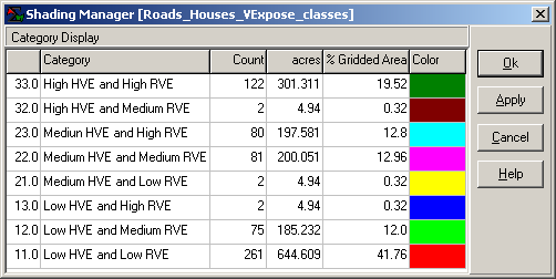
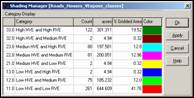 Use the Shading
Manager to label each of visual exposure combinations. For example, the 11 value is interpreted as
condition class “one-one” (Low, Low) derived by adding a 10= Low Housing_VExpose_class plus 1= Low Roads_VExpose_class.
Use the Shading
Manager to label each of visual exposure combinations. For example, the 11 value is interpreted as
condition class “one-one” (Low, Low) derived by adding a 10= Low Housing_VExpose_class plus 1= Low Roads_VExpose_class.
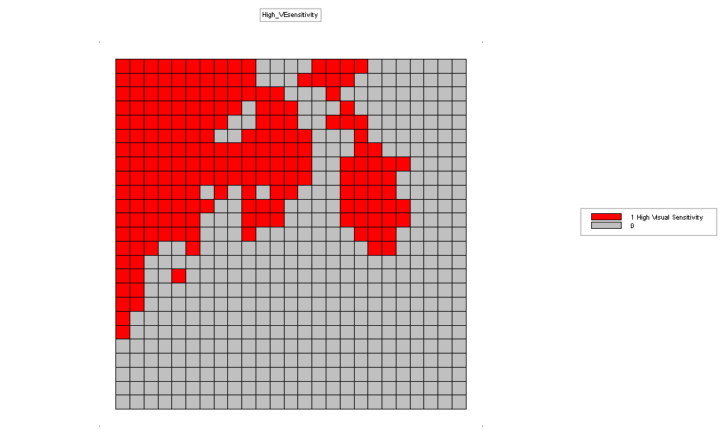
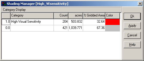
Isolate the visually
sensitive areas by selecting Map
Analysisà Reclassifyà Renumber
and completing the dialog box as shown.
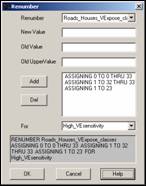 RENUMBER Roads_Houses_VExpose_classes ASSIGNING 0 TO 0 THRU
33 ASSIGNING 1 TO 32 THRU 33 ASSIGNING 1 TO 23 FOR High_VEsensitivity
RENUMBER Roads_Houses_VExpose_classes ASSIGNING 0 TO 0 THRU
33 ASSIGNING 1 TO 32 THRU 33 ASSIGNING 1 TO 23 FOR High_VEsensitivity


Note that about a third of
the project area is visually vulnerable and is concentrated in the northwestern
portion of the area. “Ugly” development
or activities ought to avoid these areas.
On your own, follow a similar
visual analysis procedure to generate a map that identifies visual exposure
classes to water (Water map) and
forest cover (Covertype map). What percent of the project area has high
visual exposure to water and forest combined?
“Pretty” areas like these might be potential areas for hiking trails or
that new cabin you have wanted to build.
5.6 Extending Visual Analysis to Other Areas
Click on the Map Analysis button and select Scriptà Save As…
and specify a file name for the command script such as Tutor25_exercises_5.scr.
This will save all of your work so you can re-access the command file at
a later date by selecting Map Analysisà Scriptà Openà Tutor25_exercises_5.scr.
To save the database, from
the main menu select Fileà Save As…
and save the file under a different name than the basic Tutor25.rgs name, such as Tutor25_exercises_5.rgs.
 Click on the Open existing file button and respond No to whether you want to save changes to the existing
database.
Click on the Open existing file button and respond No to whether you want to save changes to the existing
database.
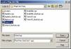 Select the Island.rgs database from the list and click Open.


Using the Elevation surface and Roads map create a Viewshed map identifying all locations that can be seen (at least
once) from the road network.

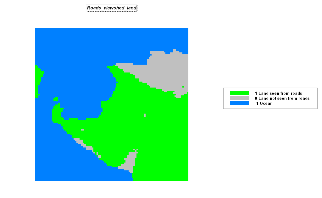
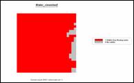
Use the Land_mask map and the Map
Analysisà Reclassifyà Cover operation
to enter the command…
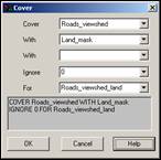 COVER Roads_viewshed WITH Land_mask IGNORE 0 FOR
Roads_viewshed_land
COVER Roads_viewshed WITH Land_mask IGNORE 0 FOR
Roads_viewshed_land

What percent of the project
area is classified as “land seen from roads.”
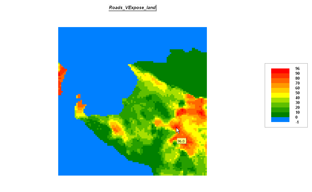
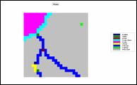
Repeat the procedure calculating
a Visual Exposure map from
roads. Display the map using User
Defined calculation mode for ranges from -1
to 0, 0 to 10, 10 to 20,…,90 to 96.
Assign blue to -1 to 0, green
to 0 to 10, yellow to 40 to 50 and red to 90 to 96.


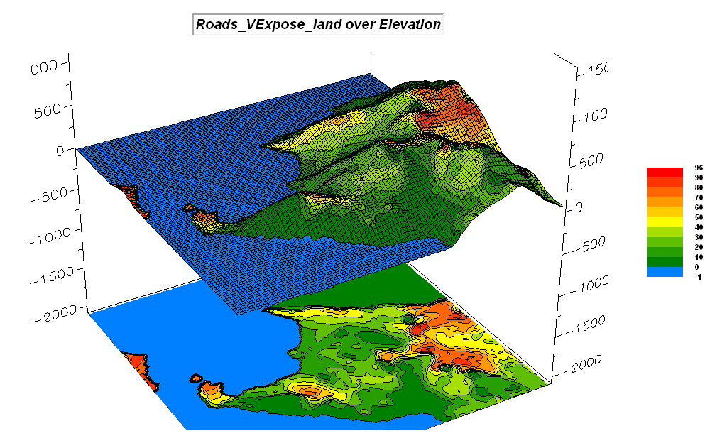
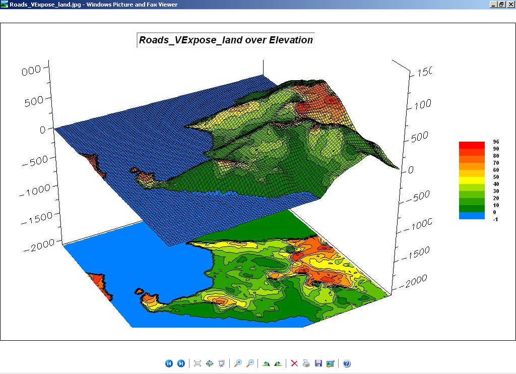
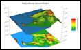
Create a more interesting
display by draping the visual exposure map over a 3-dimension plot of the
terrain by—
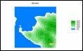
 Use the View
button (binocular icon) to display the Elevation
map.
Use the View
button (binocular icon) to display the Elevation
map.
 Use the Toggle
3D view button to switch the display to a 3-dimensional plot.
Use the Toggle
3D view button to switch the display to a 3-dimensional plot.
 From the main menu select Mapà Overlayà Roads_VExpose_land
to superimpose the visual exposure map on the Elevation surface.
From the main menu select Mapà Overlayà Roads_VExpose_land
to superimpose the visual exposure map on the Elevation surface.
 Select the Zoom Out tool (magnifying glass with minus sign), click/drag
up/down anywhere on the display to size the plot. Use the Move
tool (hand) and click/drag to center the plot.
Select the Zoom Out tool (magnifying glass with minus sign), click/drag
up/down anywhere on the display to size the plot. Use the Move
tool (hand) and click/drag to center the plot.

 Use the Save
picture of map button to capture a “screen grab” of the display as a file
named FancyMap_graphic.jpg.
Use the Save
picture of map button to capture a “screen grab” of the display as a file
named FancyMap_graphic.jpg.
Use Windows Explorer to browse to the saved file and double click on it
to display in your default viewer.

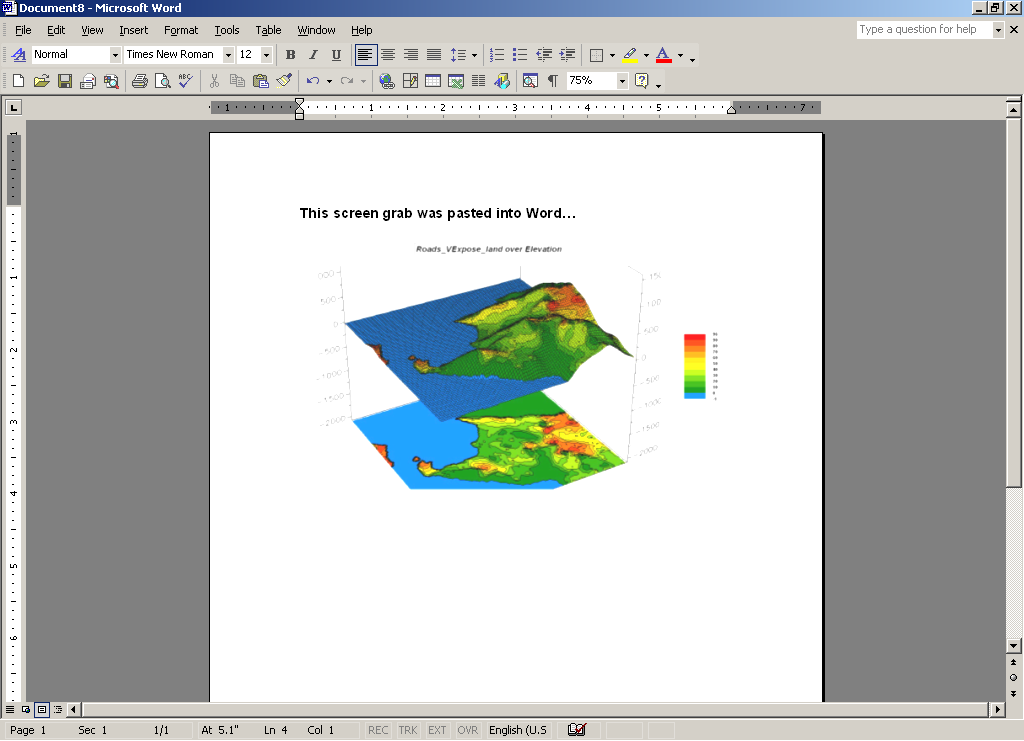
Open a blank Word document and insert the saved file
into it by—

 From the main Word menu select Insertà Pictureà From File…
and browsing to the saved file.
From the main Word menu select Insertà Pictureà From File…
and browsing to the saved file.

Note: The MapCalc
“Save picture of map” button
provides basic screen grab capability of just the map window. Microsoft Windows “Ctrl/Print Screen” capability grabs the
entire computer screen. The inexpensive
yet versatile SnagIt program provides advanced screen capture
capabilities and was used to capture/insert all of the graphics used in this
book. To order, see…www.techsmith.com/
__________________________

 Exercise 5.1
Calculating Viewsheds — in
this exercise you will first create a map of all the water locations (viewer
map) in the Tutor25 database and then generate a simple viewshed map that
indicates the visual connectivity to water— all locations are identified as
either 0= not seen or 1= seen from at least one water location.
Exercise 5.1
Calculating Viewsheds — in
this exercise you will first create a map of all the water locations (viewer
map) in the Tutor25 database and then generate a simple viewshed map that
indicates the visual connectivity to water— all locations are identified as
either 0= not seen or 1= seen from at least one water location.

 Exercise 5.2
Calculating Visual Exposure — this exercise
demonstrates generating a visual exposure map to water indicating the number
water locations visually connected to each grid location in a project area— 0=
not seen with increasing values indicating higher visual exposure to water.
Exercise 5.2
Calculating Visual Exposure — this exercise
demonstrates generating a visual exposure map to water indicating the number
water locations visually connected to each grid location in a project area— 0=
not seen with increasing values indicating higher visual exposure to water. 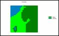
 Exercise 5.3
Accounting for Screens — this
exercise extends the previous exercise to create another visual exposure map to
water that accounts for a screening forest canopy of 75 feet and then compares
the result to the “non-screened” solution to determine the differences in the
two approaches.
Exercise 5.3
Accounting for Screens — this
exercise extends the previous exercise to create another visual exposure map to
water that accounts for a screening forest canopy of 75 feet and then compares
the result to the “non-screened” solution to determine the differences in the
two approaches.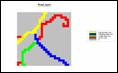
 Exercise 5.4
Calculating Weighted Visual Exposure — this
exercise first calibrates Roads in terms of traffic flow and then creates a
weighted visual exposure map accounting for the relative amount of traffic on
different road types— 0= not seen from any road location with increasing values
indicating higher weighted visual exposure to traffic flows.
Exercise 5.4
Calculating Weighted Visual Exposure — this
exercise first calibrates Roads in terms of traffic flow and then creates a
weighted visual exposure map accounting for the relative amount of traffic on
different road types— 0= not seen from any road location with increasing values
indicating higher weighted visual exposure to traffic flows. 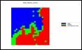
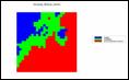
 Exercise 5.5
Modeling Visual Exposure Impacts — this exercise
creates and classifies visual exposure maps for relative connectivity to roads
and houses (Low, Medium, High) and then combines the two classified maps into a
single map that characterizes the joint visual exposure for each map location
using a 2-digit code— a location with a value of 11 indicates 1= Low housing
exposure and 1= Low roads exposure; a value of 12= Low/Medium, … to a value of
33= High/High.
Exercise 5.5
Modeling Visual Exposure Impacts — this exercise
creates and classifies visual exposure maps for relative connectivity to roads
and houses (Low, Medium, High) and then combines the two classified maps into a
single map that characterizes the joint visual exposure for each map location
using a 2-digit code— a location with a value of 11 indicates 1= Low housing
exposure and 1= Low roads exposure; a value of 12= Low/Medium, … to a value of
33= High/High. 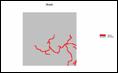
 Exercise 5.6
Extending Visual Analysis to Other Areas — this
exercise creates a visual exposure map to roads and graphically overlays it on
the Elevation surface for the Island database.
Exercise 5.6
Extending Visual Analysis to Other Areas — this
exercise creates a visual exposure map to roads and graphically overlays it on
the Elevation surface for the Island database.