|
Topic 4 –
Calculating Effective Distance |
Map
Analysis book/CD |

Extending
GIS Procedures with Variable-Width Buffers — discusses
the basic considerations in establishing variable-width buffers that respond to
both intervening conditions and the type of connectivity
Create
Effective Distance Buffers to Improve Map Accuracy — develops
procedures for creating buffers that respond to the relative ease of movement
Measuring
Distance Is Neither Here nor There — discusses the basic concepts
of distance and proximity
Extend
Simple Proximity to Effective Movement — discusses
the concept of effective distance responding to relative and absolute barriers
Further Reading
— twenty one additional sections organized into five parts
<Click here>
for a printer-friendly version of this
topic (.pdf).
(Back to the Table of Contents)
______________________________
Extending
GIS Procedures with Variable-Width Buffers
(GeoWorld, November 2000)
In
part, the graphical and inventory aspects of traditional maps have dominated
the digital translation of spatial information.
Users can enter an address and instantly view a map of that location and
print a set of driving instructions. One
can publish a couple of hundred scanned topographic sheets on a CD that can be
panned and zoomed at several scales.
Images and even streaming video can be linked to their precise locations
on a map and accessed over the web simply by clicking on an embedded symbol.
The
digital expression of familiar mapping procedures represented the first wave in
recasting
A good
example of infusing extended
Most
folks immediately recognize the shortcomings of a simple buffer. Common sense tells us that while delineating
a single “as-the-crow-flies” distance under all possible intervening conditions
might meet the letter of the law, it often violates reality. The concept of variable-width buffers that
match reality has been with us for years—what is missing is a traditional mindset
and experience with a tool. What is
needed for second wave applications is education that fosters understanding and
confidence in the extended procedures.
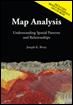
Figure
1. A Simple Proximity Buffer identifies
the distance to roads throughout the buffered area. Note that the buffer extends into the
ocean—an inappropriate “reach” for terrestrial applications.
Consider
the road network and its 250-meter Simple Proximity Buffer as
depicted in figure 1. In most desktop
mapping systems a “Buffer Tool” is used to automatically inscribe a line at a
given distance from a complex feature.
The dark blue edge of the buffer in the figure identifies this maximum
reach. However, the color progression
indicates the relative proximity within the buffer—from yellow (close) to dark
blue (far). While most folks have little
experience with a simple proximity buffer, they immediately relate to the concept
and value of the added information.
Also
they immediately see some of its limitations.
Notice how the consistent reach causes the buffer to extend into
unintended areas—the ocean in this case.
The “geographic slop” is more than graphically troublesome; it can skew
statistics and misrepresent spatial relationships for terrestrial applications.
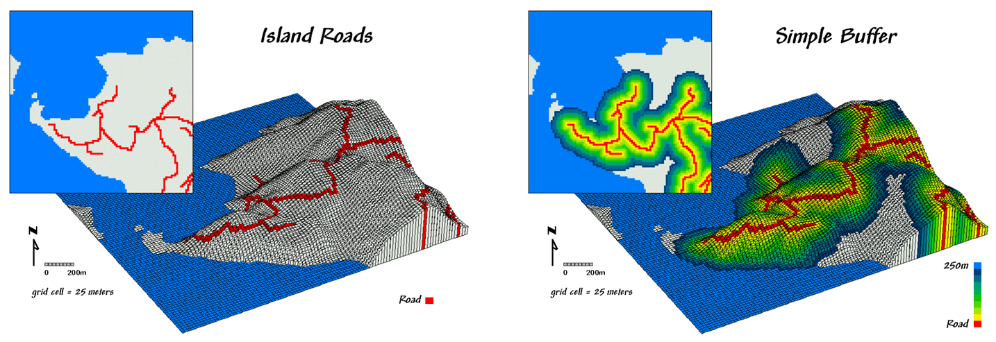
Figure
2. The figure on the left clips the
simple buffer to represent only land areas.
The figure on the right uses the elevation surface to identify only
areas that are uphill from the roads.
The
left side of figure 2 shows a Clipped Buffer, the first
conceptual step toward variable-width buffers.
Some
For
example, consider the Uphill Buffer maps on the right side of
figure 2. In this instance the measurement
of proximity for the buffered area was forced to extend only “uphill” from the
roads as defined on a guiding surface (a short conceptual step from a masking
map). The results when draped over the
elevation surface confirm that only uphill locations are identified. By simply specifying “downhill” only those
locations that are below the roads (and not within in the ocean mask) would be
identified.
The
division of a simple buffer into its uphill and downhill components can be
important. A road engineer sees
different land slippage considerations in the two areas. An environmental scientist concentrates on
the downhill portion for flows of oil and other chemicals from the road. In fact in most applications consideration
of the characteristics and conditions within a buffer are at least as important
as the outline of its extent.
The
ability to establish proximity-based buffers that react to geographic
conditions isn’t part of our paper map legacy.
However, the concept is ingrained in practical experience. As subsequent columns in this mini-series
will show, the ability to identify up/downwind buffers, noise attenuation
buffers, customer travel-time buffers and other effective proximity buffers
that respond to geographic conditions are no longer beyond our reach. The tools are at hand (and actually have been
for quite some time). What waits is a
second wave of innovative applications that take advantage of the new tools and
instill their commonplace acceptance.
Create
Effective Distance Buffers to Improve Map Accuracy
(GeoWorld, January 2001)
One of
the most fundamental operations in
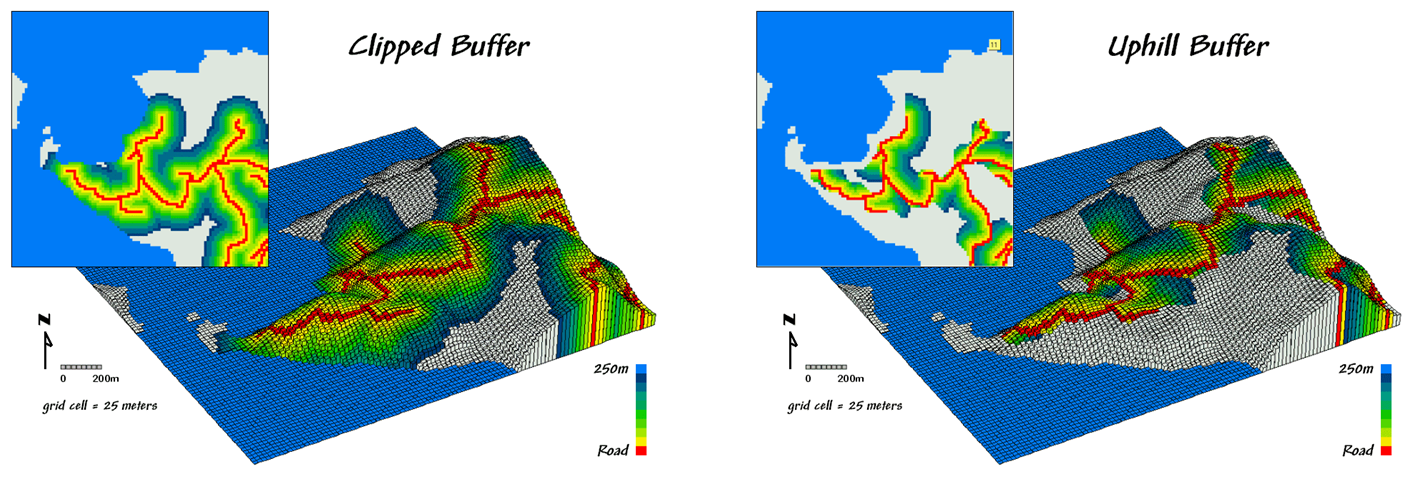
Figure
1, on the other hand, shows some of the extensions to traditional buffering that
were discussed in the past couple of columns.
Inset a) characterizes the relative proximity of all locations
within a road buffer of 250 meters.
Inset b) clips the road buffer for infeasible areas, such as open
water. A buffer identifying just the uphill
areas from the road is shown in inset c). Insets d) and e) characterize
the locations within 250 meters that can be seen from the road network (Viewshed)
and their relative amount of visual exposure (Expose).
Inset f)
shows the proximity to the road for areas within the viewshed buffer. This information can be useful in determining
visual impact—locations that are seen a lot and are near roads equate to high
visual impact. Similarly, noise
dissipation can be coarsely modeled as inversely related to line-of-sight
distance—it’s fairly quiet at locations that are relatively near the road but
on the other side of a ridge (outside the line-of-sight buffer).
The
previous discussions should have you rethinking the utility of scribing lines that
are “everywhere-the-same” in characterizing the influences about a map
feature. In the real world, spatial
context is rarely as simple as implied by the lines of a traditional buffer.
For
example, consider hiking in mountainous terrain. In gentle terrain you move along at a brisk
pace. But as the terrain becomes
steeper, progress slows until eventually there are slopes that repels most
hikers (no pun intended). It is common
sense that steep intervening conditions can make locations “effectively” farther
away. Conversely, gentle intervening
slopes make locations much more accessible.
Figure
1. Examples of Variable-Width and Line-of-Sight
Buffers.
The
effect of slope on defining a buffer’s reach is developed in Figure 2. The top left inset is a map of the slope
conditions from 0 to 100 percent. The Hiking_Friction
map calibrates the slopes in terms of the relative ease of foot-travel— 0-5%
Easy, 5-10% Moderate, 10-20% Hard, 20-40% Difficult, and >40% a no-go
situation.
It is
important to note that the value 1 is assigned to the easiest conditions to
cross and all other slope conditions are assigned a value indicating increased
difficulty— 2= twice as hard, 5= five times as hard, 10= ten times as hard and
–2 for inaccessible no-go areas.
Calibration
of these values relate to the relative “cost” of traversing a grid cell and in
this instance it was assumed to take 15 seconds to cross the easiest 25 meter
cell. A moderate cell, on the other
hand, is twice as difficult and takes 30 seconds to cross; a hard cell takes 75
seconds (1.25 minutes); and a difficult cell takes 250 seconds (4.17 minutes). An effective-distance operation is used that
extends and contacts the width of the buffer considering the intervening
conditions as calibrated on the friction map (Hiking_Buffer inset in
figure 2).
In this
instance, an effective buffer reach of 50 cells was used. If the road were surrounded completely by
gentle slopes, the buffer would extend a consistent 50 cells from all locations
and have the appearance of a traditional buffer. However, as steeper areas are encountered the
geographic reach is shortened. In fact
the portion of the road in the lower right of the map is surrounded by “no-go”
conditions and the buffer is truncated at the edge of the road.
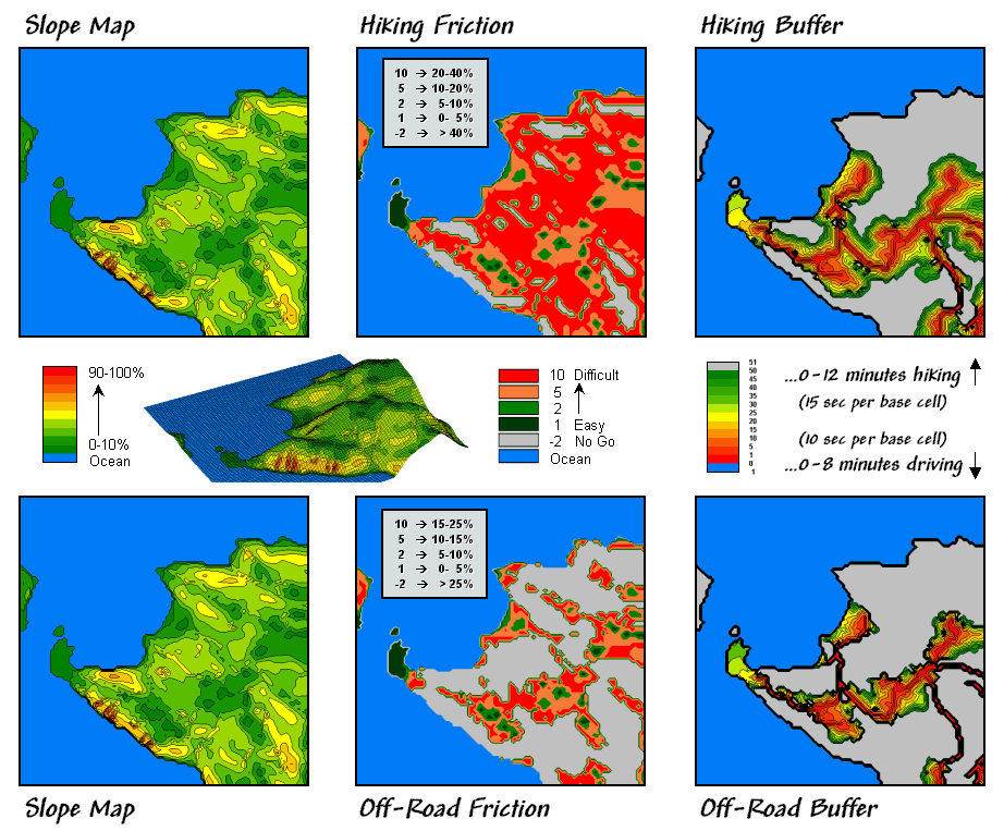
Figure
2. Development of Effective-Distance
Buffers for Hiking and off-road travel.
The
lower set of maps in figure 2 repeats the analysis to create an
effective-distance buffer assuming vehicular off-road travel. The slope map was calibrated for off-road
travel assuming an 10 second base friction for the gentle slopes (0-5%); 20
seconds for 5-10%; 50 seconds for 10-15%; 100 seconds (1.7 minutes) for 15-25%;
and >25% a no-go situation. Note the
extensive area of inaccessible regions identified in the Off-Road_Friction
map giving the buffer a spindly look.
Now
compare the hiking and off-road buffers based on effective-distance. A significantly larger portion of the Off-Road_Buffer
is classified as inaccessible. An
effective reach of 50 cells is used in both cases, but the calibration
generates a 0 to 12 minute buffer for hiking and a 0 to 8 minute buffer for an
off-road vehicle. In both instances, the
effective buffers are radically different from that of a traditional fixed-width
buffer and provide considerable more information about relative movement within
the buffered area.
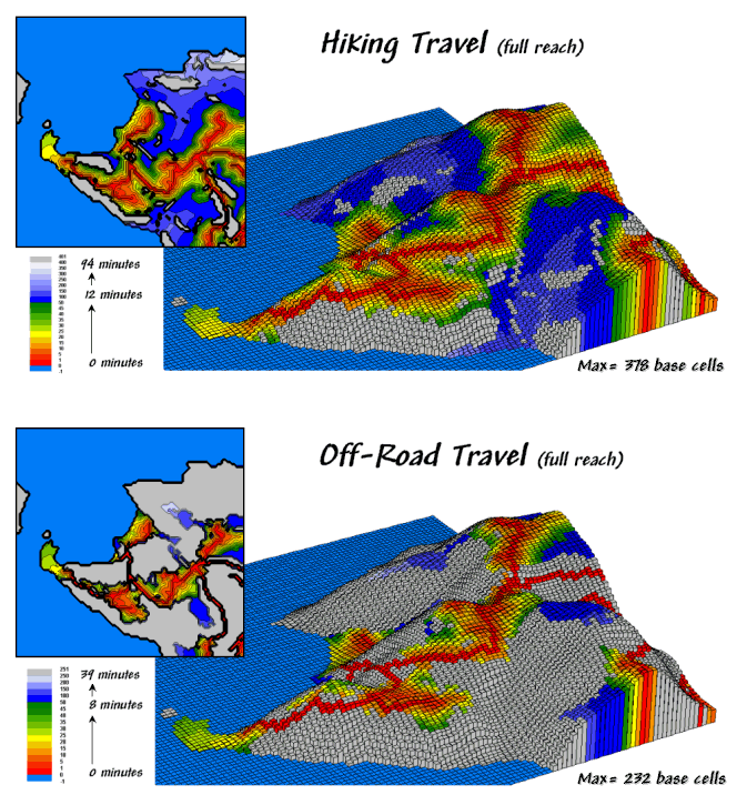
Figure
3. Comprehensive Travel-Time Maps for
Hiking and Off-Road Movement.
Figure
3 literally extends the processing a bit farther by increasing the reach to encompass
all accessible areas by hiking or off-road travel. The blue tones on each map identify
incrementally larger reaches beyond the buffers shown in figure 2. Note that the areas reached by off-road
travel are significantly less than those reached by hiking.
Also
note the extended reach shown for the area in the lower right portion of
project. The off-road travel map extends
along a relatively gentle ridge but stops abruptly as the slopes exceed 25%. The hiking travel map, on the other hand, extends
along the ridge and clear to the ocean.
The gray tones indicate areas that are beyond reach (inaccessible) and
can occur as pockets. The farthest
location for a hiker is 94 minutes (378 effective cells) and for a off-road
vehicle, is 39 minutes (232 effective cells).
One’s
first encounter with variable-width buffers might seem a bit uncomfortable
since we can’t create them with a ruler, but the concept aligns with common
sense. A traditional buffer makes the
broad assumption that the reach is everywhere the same. The different types of variable-width buffers
reject this assumption and attempt to characterize the intervening conditions
and their affects on the buffer’s reach.
Of
course the accuracy of the new buffers depends on the exactness of the
ancillary data and the algorithms underlying the enabling map analysis
operations. However, in most
applications the inherent inaccuracy of the underlying assumption of
traditional buffers far outweighs these concerns—a simple buffer is most often
simply wrong.
Measuring Distance Is Neither Here nor There
(GeoWorld, April 2005)
Measuring
distance is one of the most basic map analysis techniques. Historically, distance is defined as the shortest straight-line
between two points. While
this three-part definition is both easily conceptualized and implemented with a
ruler, it is frequently insufficient for decision-making. A straight-line route might indicate the
distance “as the crow flies,” but offer little information for the walking crow
or other flightless creature. It is
equally important to most travelers to have the measurement of distance
expressed in more relevant terms, such as time or cost.
The
limitation of a map analysis approach is not so much in the concept of distance
measurement, but in its implementation.
Any measurement system requires two components— a standard unit and a procedure for measurement.
Using a ruler, the “unit” is the smallest hatching along its edge and
the “procedure” is the line implied by aligning the straightedge. In effect, the ruler represents just one row
of a grid implied to cover the entire map.
You just position the grid such that it aligns with the two points you
want measured and count the squares (top portion of figure 1). To measure another distance you merely
realign the implied grid and count again.
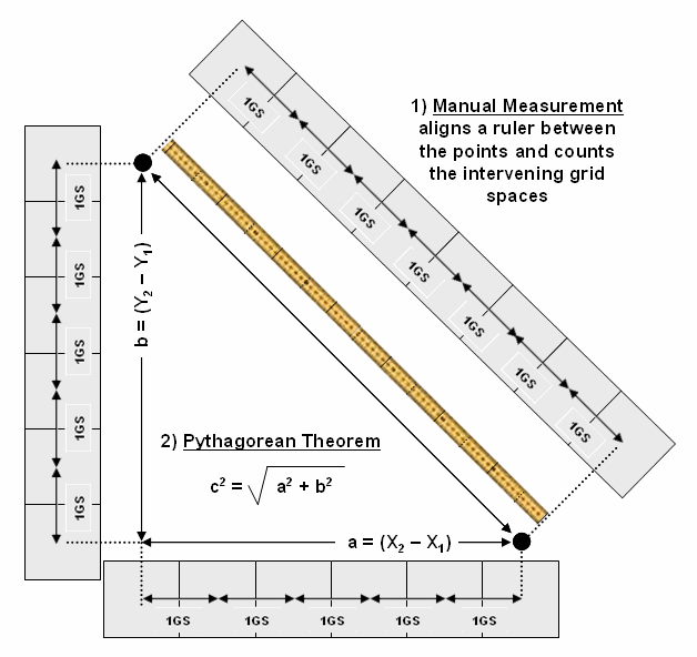
Figure 1. Both Manual Measurement and the Pythagorean
Theorem use grid spaces as the fundamental units for determining the distance
between two points.
In a
Proximity
establishes the distance to all locations surrounding a point— the set of shortest straight-lines
among groups of points.
Rather than sequentially computing the distance between pairs of
locations, concentric equidistance zones are established around a location or
set of locations (figure 2). This
procedure is similar to the wave pattern generated when a rock is thrown into a
still pond. Each ring indicates one
“unit farther away”— increasing distance as the wave moves away. Another way to conceptualize the process is
nailing one end of a ruler at a point and spinning it around. The result is a series of “data zones”
emanating from a location and aligning with the ruler’s tic marks.
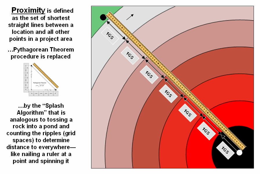
Figure 2. Proximity identifies the set of shortest
straight-lines among groups of points (distance zones).
However,
nothing says proximity must be measured from a single point. A more complex proximity map would be
generated if, for example, all locations with houses (set of points) are
simultaneously considered target locations (right side of figure 3).
In
effect, the procedure is like throwing a handful of rocks into pond. Each set of concentric rings grows until the
wave fronts meet; then they stop. The
result is a map indicating the shortest straight-line distance to the nearest
target location (house) for each non-target location. In the figure, the red tones indicate locations
that are close to a house, while the green tones identify areas that are far
from a house.
In a
similar fashion, a proximity map to roads is generated by establishing data
zones emanating from the road network—sort of like tossing a wire frame into a
pond to generate a concentric pattern of ripples (middle portion of figure
3). The same result is generated for a
set of areal features, such as sensitive habitat parcels (right side of figure
3).
It is
important to note that proximity is not the same as a buffer. A buffer is a discrete spatial object that
identifies areas that are within a specified distance of map feature; all
locations within a buffer are considered the same. Proximity is a continuous surface that
identifies the distance to a map feature(s) for every location in a project
area. It forms a gradient of distances
away composed of many map values; not a single spatial object with one
characteristic distance away.
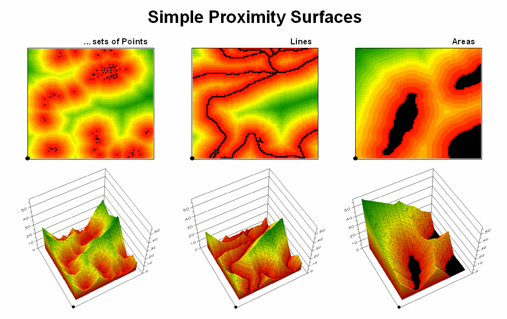
Figure 3. Proximity surfaces can be generated for
groups of points, lines or polygons identifying the shortest distance from all
location to the closest occurrence.
The 3D
plots of the proximity surfaces in figure 3 show detailed gradient data and are
termed accumulated surfaces. They contain increasing distance values from
the target point, line or area locations displayed as colors from red (close)
to green (far).
The
starting features are the lowest locations (black= 0) with hillsides of
increasing distance and forming ridges that are equidistant from starting
locations. Next month will focus on how
proximity is calculated—conceptually easy but way too much bookkeeping for even
the most ardent accountant.
Extend Simple Proximity to Effective Movement
(GeoWorld, June 2005)
Last
section’s discussion suggested that in many applications, the shortest route
between two locations might not always be a straight-line. And even if it is straight, its geographic
length may not always reflect a traditional measure of distance. Rather, distance in these applications is
best defined in terms of “movement” expressed as travel-time, cost or energy
that is consumed at rates that vary over time and space. Distance modifying effects involve weights
and/or barriers— concepts that imply the relative ease of movement through
geographic space might not always constant.
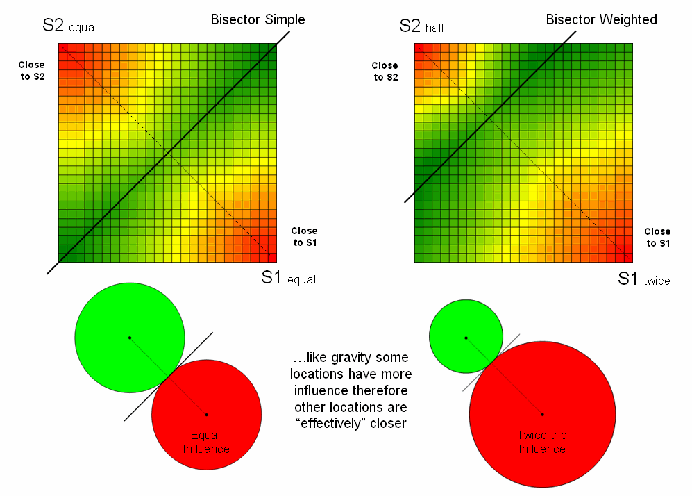
Figure 1. Weighting factors based on the
characteristics of movement can affect relative distance, such as in Gravity
Modeling where some starting locations exert more influence.
Figure
1 illustrates one of the effects of distance being affected by a movement characteristic. The left-side of the figure shows the simple
proximity map generated when both starting locations are considered to have the
same characteristics or influence. Note
that the midpoint (dark green) aligns with the perpendicular bisector of the
line connecting the two points and confirms a plane geometry principle you learned
in junior high school.
The
right-side of the figure, on the other hand, depicts effective proximity where
the two starting locations have different characteristics. For example, one store might be considered
more popular and a “bigger draw” than another (Gravity Modeling). Or in old geometry terms, the person starting
at S1 hikes twice as fast as the individual starting at S2— the weighted
bisector identifies where they would meet.
Other examples of weights include attrition where movement changes with
time (e.g., hiker fatigue) and change in mode (drive a vehicle as far as
possible then hike into the off-road areas).
In
addition to weights that reflect movement characteristics, effective proximity
responds to intervening conditions or barriers. There are two types of barriers
that are identified by their effects— absolute and relative. Absolute
barriers are those completely restricting movement and therefore imply an
infinite distance between the points they separate. A river might be regarded as an absolute
barrier to a non-swimmer. To a swimmer
or a boater, however, the same river might be regarded as a relative barrier identifying areas that
are passable, but only at a cost which can be equated to an increase in
geographical distance. For example, it
might take five times longer to row a hundred meters than to walk that same
distance.
In the
conceptual framework of tossing a rock into a pond, the waves can crash and
dissipate against a jetty extending into the pond (absolute barrier; no
movement through the grid spaces). Or
they can proceed, but at a reduced wavelength through an oil slick (relative
barrier; higher cost of movement through the grid spaces). The waves move both around the jetty and
through the oil slick with the ones reaching each location first identifying the set of shortest, but not
necessarily straight-lines among groups of points.
The
shortest routes respecting these barriers are often twisted paths around and
through the barriers. The
For
example, figure 2 shows the effective proximity surfaces for the same set of
starter locations discussed in the first section in this topic. The point features in the left inset respond
to treating flowing water as an absolute barrier to movement. Note that the distance to the nearest house
is very large in the center-right portion of the project area (green) although
there is a large cluster of houses just to the north. Since the water feature can’t be crossed, the
closest houses are a long distance to the south.
Terrain
steepness is used in the middle inset to illustrate the effects of a relative
barrier. Increasing slope is coded into
a friction map of increasing impedance values that make movement through steep
grid cells effectively farther away than movement through gently sloped
locations. Both absolute and relative
barriers are applied in determining effective proximity sensitive areas in the
right inset.
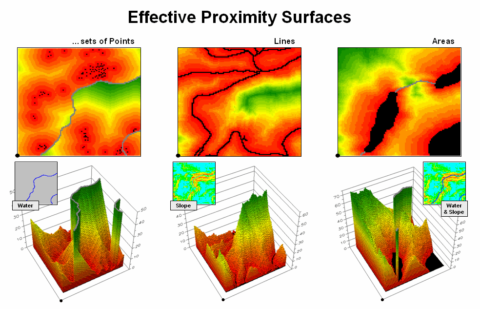
Figure 2. Effective Proximity surfaces consider the
characteristics and conditions of movement throughout a project area.
The
dramatic differences between the concept of distance “as the crow flies”
(simple proximity) and “as the crow walks” (effective proximity) is a bit
unfamiliar and counter-intuitive.
However, in most practical applications, the comfortable assumption that
all movement occurs in straight lines totally disregards reality. When traveling by trains, planes,
automobiles, and feet there are plenty of bends, twists, accelerations and decelerations
due to characteristics (weights) and conditions (barriers) of the
movement.
Figure
3 illustrates how the splash algorithm propagates distance waves to generate an
effective proximity surface. The
Friction Map locates the absolute (blue/water) and relative (light blue=
gentle/easy through red= steep/hard) barriers.
As the distance wave encounters the barriers their effects on movement
are incorporated and distort the symmetric pattern of simple proximity waves. The result identifies the “shortest, but not
necessarily straight” distance connecting the starting location with all other
locations in a project area.
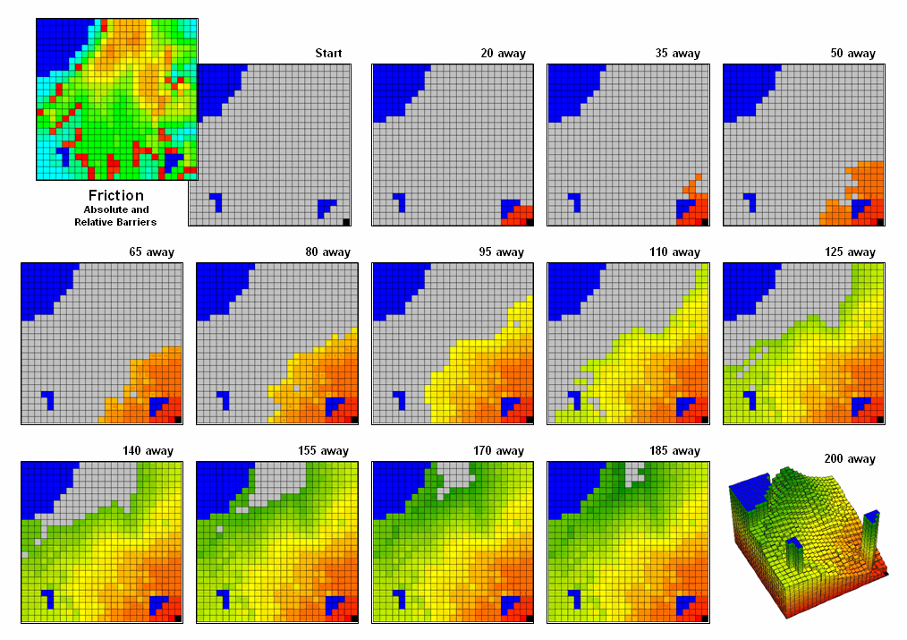
Figure 3. Effective Distance
waves are distorted as they encounter absolute and relative barriers, advancing
faster under easy conditions and slower in difficult areas.
Note
that the absolute barrier locations (blue) are set to infinitely far away and
appear as pillars in the 3-D display of the final proximity surface. As with simple proximity, the effective
distance values form a bowl-like surface with the starting location at the
lowest point (zero away from itself) and then ever-increasing distances away
(upward slope).
With
effective proximity, however, the bowl is not symmetrical and is warped with
bumps and ridges that reflect intervening conditions— the greater the impedance
the greater the upward slope of the bowl.
In addition, there can never be a depression as that would indicate a
location that is closer to the starting location than everywhere around
it. Such a situation would violate the
ever-increasing concentric rings theory and is impossible except on Star Trek
where Spock and the Captain de-materialize then reappear somewhere else without
physically passing through the intervening locations.
_____________________
Further Online
Reading: (Chronological
listing posted at www.innovativegis.com/basis/BeyondMappingSeries/)
(Calculating Simple and Effective Proximity)
Use Cells and Rings to Calculate
Simple Proximity — describes how simple proximity is calculated (May
2005)
Calculate and Compare to Find
Effective Proximity — describes how effective proximity is
calculated (July 2005)
Taking Distance to the Edge
— discusses advance distance operations (August 2005)
(Deriving and Analyzing Travel-Time)
Use Travel-Time Buffers to Map
Effective Proximity — discusses procedures for
establishing travel-time buffers responding to street type (February 2001)
Integrate Travel-Time into Mapping
Packages — describes procedures for transferring
travel-time data to other maps (March 2001)
Derive and Use Hiking-Time Maps for
Off-Road Travel — discusses procedures for
establishing hiking-time buffers responding to off-road travel (April
2001)
Consider Slope and Scenic Beauty in
Deriving Hiking Maps — describes a general
procedure for weighting friction maps to reflect different objectives (May
2001)
Accumulation Surfaces Connect Bus Riders
and Stops — discusses an accumulation surface analysis procedure
for linking riders with bus stops (October 2002)
(Use of Travel-Time in Geo-Business)
Use Travel Time to Identify Competition
Zones — discusses the procedure for deriving relative travel-time
advantage maps (March 2002)
Maps and Curves Can Spatially
Characterize Customer Loyalty — describes a
technique for characterizing customer sensitivity to travel-time (April
2002)
Use Travel Time to Connect with
Customers — describes techniques for optimal path and catchment
analysis (June 2002)
GIS Analyzes In-Store Movement and
Sales Patterns — describes a procedure using
accumulation surface analysis to infer shopper movement from cash register data (February
1998)
Further Analyzing In-Store Movement
and Sales Patterns — discusses how map analysis is
used to investigate the relationship between shopper movement and sales (March
1998)
Continued Analysis of In-Store
Movement and Sales Patterns — describes the use of
temporal analysis and coincidence mapping to enhance shopping patterns (April
1998)
(Micro-Terrain Considerations and Techniques)
Confluence Maps Further Characterize
Micro-terrain Features — describes the use of optimal path
density analysis for mapping surface flows (April 2000)
Modeling Erosion and Sediment
Loading — illustrates a
Identify Valley Bottoms in
Mountainous Terrain — illustrates a technique for
identifying flat areas connected to streams (November 2002)
(Surface Flow Considerations and Techniques)
Traditional Approaches Can’t
Characterize Overland Flow — describes the basic considerations in
overland flow (November 2003)
Constructing Realistic Downhill
Flows Proves Difficult — discusses procedures for characterizing
path, sheet, horizontal and fill flows (December 2003)
Use Available Tools to Calculate
Flow Time and Quantity — discusses procedures for tracking flow
time and quantity (January 2004)
Migration Modeling Determines Spill
Effect — describes procedures for assessing
overland and channel flow impacts (February 2004)