|
Beyond
Mapping IV Topic 9
– Math/Stat Framework for Map Analysis (Further Reading) |
GIS Modeling book |
Map-ematically
Messing with Mapped Data — discusses the nature of grid-based
mapped data and Spatial Analysis operations (February 2012)
Paint
by Numbers Outside the Traditional Statistics Box
— discusses the nature of Spatial Statistics operations (March 2012)
The
Spatial Key to Seeing the Big Picture — describes a five step
process for generating grid map layers from spatially tagged data (September 2013)
Recasting
Map Analysis Operations for General Consumption — reorganizes ArcGIS’s
Spatial Analyst tools into the SpatialSTEM framework that extends traditional
math/stat procedures (February 2013)
<Click here> for a printer-friendly version of this topic (.pdf).
(Back
to the Table of Contents)
______________________________
Map-ematically Messing with Mapped Data
(GeoWorld,
February 2012)
Earlier discussion introduced the idea of spatialSTEM for teaching
map analysis and modeling fundamentals within a mathematical context that
resonates with science, technology, engineering and math/stat communities (“SpatialSTEM
Has Deep Mathematical Roots,” GeoWorld, January 2012 ). The discussion established a general
framework and grid-based data structure needed for quantitative analysis of
spatial patterns and relationships. This
section focuses on the nature of mapped data, an example of a grid-math/algebra
application and discussion of extended spatial analysis operations.
Figure 1 identifies the two primary perspectives of spatial data—1) Numeric
that indicates how numbers are distributed in “number space” (What
condition) and 2) Geographic that indicated how numbers are distributed
in “geographic space” (Where condition).
The numeric perspective can be grouped into categories of Qualitative
numbers that deal with general descriptions based on perceived “quality” and Quantitative
numbers that deal with measured characteristics or “quantity.”
Further classification identifies the familiar numeric data types of
Nominal, Ordinal, Interval, Ratio and Binary.
It is generally well known that very few math/stat operations can be
performed using qualitative data (Nominal, Ordinal), whereas a wealth of
operations can be used with quantitative data (Interval, Ratio). Only a specialized few operations utilize
Binary data.
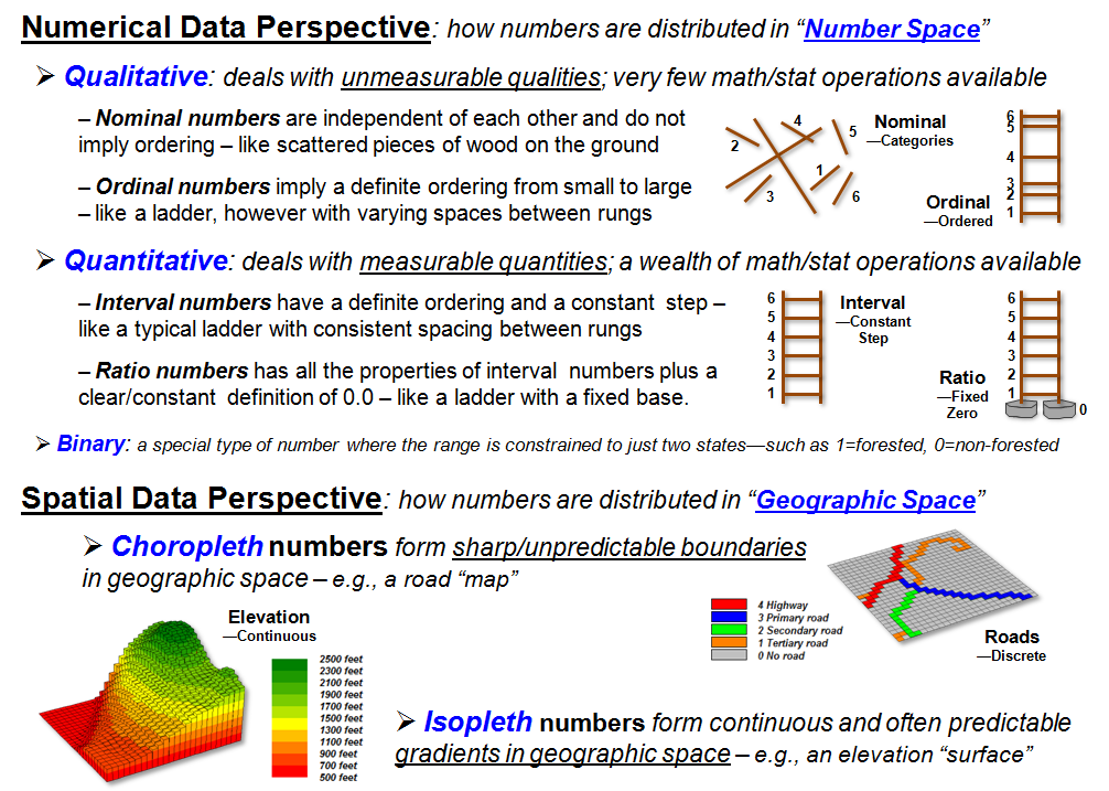
Figure 1. Spatial Data Perspectives—Where
is What.
Less familiar are the two geographic data types. Choropleth numbers form sharp and unpredictable
boundaries in space, such as the values assigned to the discrete map features
on a road or cover type map. Isopleth
numbers, on the other hand, form continuous and often predictable gradients in
geographic space, such as the values on an elevation or temperature
surface.
Putting the Where and What perspectives of spatial data together, Discrete
Maps identify mapped data with spatially independent numbers
(qualitative or quantitative) forming sharp abrupt boundaries (choropleth),
such as a cover type map. Discrete maps
generally provide limited footholds for quantitative map analysis. On the other hand, Continuous Maps contain
a range of values (quantitative only) that form spatial gradients (isopleth),
such as an elevation surface. They provide
a wealth of analytics from basic grid math to map algebra, calculus and
geometry.
Site-specific farming provides a good example of basic grid math and
map algebra using continuous maps (figure 2).
Yield Mapping involves simultaneously recording yield flow and
GPS position as a combine harvests a crop resulting in a grid map of thousands
of geo-registered numbers that track crop yield throughout a field. Grid Math can be used to calculate
the mathematical difference in yield at each location between two years by
simply subtracting the respective yield maps.
Map Algebra extends the processing by spatially evaluating the
full algebraic percent change equation.
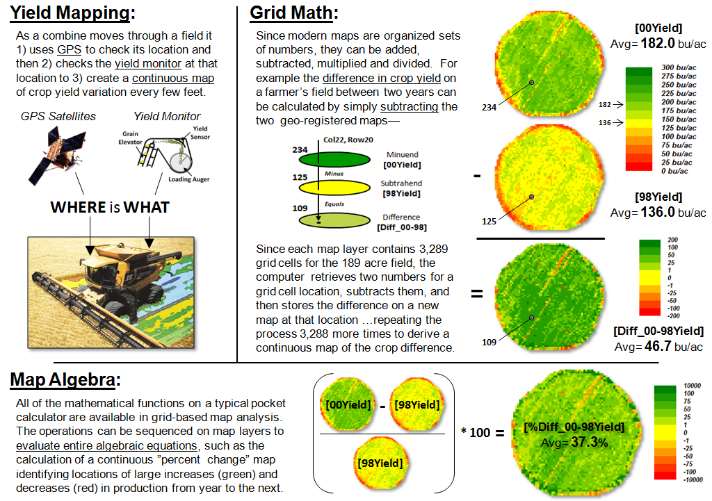
Figure 2. Basic Grid Math
and Algebra example.
The paradigm shift in this map-ematical
approach is that map variables, comprised of thousands of geo-registered
numbers, are substituted for traditional variables defined by only a single
value. Map algebra’s continuous map
solution shows localized variation, rather than a single “typical” value being
calculated (i.e., 37.3% increase in the example) and assumed everywhere the
same in non-spatial analysis.
Figure 3 expands basic Grid Math and Map Algebra into other
mathematical arenas. Advanced Grid
Math includes most of the buttons on a scientific calculator to include
trigonometric functions. For example,
taking the cosine of a slope map expressed in degrees and multiplying it times
the planimetric surface area of a grid cell calculates the surface area of the
“inclined plane” at each grid location.
The difference between planimetric area represented by traditional maps
and surface area based on terrain steepness can be dramatic and greatly affect
the characterization of “catchment areas” in environmental and engineering
models of surface runoff.
A Map Calculus expresses such functions as the derivative and
integral within a spatial context. The derivative
traditionally identifies a
measure of how a mathematical function changes as its input changes by
assessing the slope along a curve in 2-dimensional abstract space.
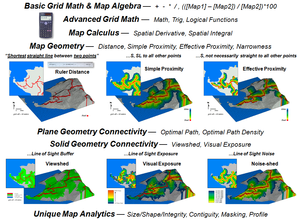
Figure 3.
Spatial Analysis operations.
The spatial equivalent calculates a “slope map” depicting the rate of
change in a continuous map variable in 3-dimensional geographic space. For an elevation surface, slope depicts the
rate of change in elevation. For an
accumulation cost surface, its slope map represents the rate of change in cost
(i.e., a marginal cost map). For a
travel-time accumulation surface, its slope map indicates the relative change
in speed and its aspect map identifies the direction of optimal movement at
each location. Also, the slope map of an
existing topographic slope map (i.e., second derivative) will characterize
surface roughness (i.e., areas where slope itself is changing).
Traditional calculus identifies an integral as the net signed area of a region along a curve expressing a mathematical function. In a somewhat analogous procedure, areas
under portions of continuous map
surfaces can be characterized. For
example, the total area (planimetric or surface) within a series of watersheds can be
calculated; or the total tax revenue for various neighborhoods; or the total
carbon emissions along major highways; or the net difference in crop yield for
various soil types in a field. In the
spatial integral, the net sum of the numeric values for portions of a
continuous map surface (3D) is calculated in a manner comparable to calculating
the area under a curve (2D).
Traditional geometry defines Distance as “the shortest
straight line between two points” and routinely measures it with a ruler or
calculates it using the Pythagorean Theorem.
Map Geometry extends the concept of distance to Simple Proximity
by relaxing the requirement of just “two points” for distances to all
locations surrounding a point or
other map feature, such as a road.
A further extension involves Effective Proximity that relaxes “straight
line” to consider absolute and relative barriers to movement. For example effective proximity might consider
just uphill locations along a road or a complex set of variable hiking
conditions that impede movement from a road as a function of slope, cover type
and water barriers.
The result is that the “shortest but not
necessarily straight distance” is assigned to each grid location. Because a straight line connection cannot be
assumed, optimal path routines in Plane Geometry Connectivity (2D space)
are needed to identify the actual shortest routes. Solid Geometry Connectivity (3D space)
involves line-of-sight connections that identify visual exposure among
locations. A final class of operations
involves Unique Map Analytics, such as size, shape, intactness and
contiguity of map features.
Grid-based map analysis takes us well beyond traditional mapping …as
well as taking us well beyond traditional procedures and paradigms of
mathematics. The next section considers
extension of traditional statistics to spatial statistics within the spatialSTEM
framework.
_____________________________
Author’s
Notes: a table of URL links to
further readings on the grid-based map analysis/modeling concepts, terminology,
considerations and procedures described in this three-part series on
spatialSTEM is posted at www.innovativegis.com/basis/MapAnalysis/Topic30/sSTEM/sSTEMreading.htm.
Paint by Numbers Outside
the Traditional Statistics Box
(GeoWorld, March
2012)
The previous section described a general framework and approach for
teaching spatial analysis within a mathematical context that resonates with
science, technology, engineering and math/stat communities (spatialSTEM). The following discussion focuses on extending
traditional statistics to a spatial statistics for understanding
geographic-based patterns and relationships.
Whereas Spatial analysis focuses on “contextual relationships”
in geographic space (such as effective proximity and visual exposure), Spatial
statistics focuses on “numerical relationships” within and among mapped
data (figure 1). From a spatial
statistics perspective there are three primary analytical arenas— Summaries,
Comparisons and Correlations.
Statistical summaries provide generalizations of the grid values
comprising a single map layer (within), or set of map layers (among). Most common is a tabular summary included in
a discrete map’s legend that identifies the area and proportion of occurrence
for each map category, such as extremely steep terrain comprising 286 acres (19
percent) of a project area. Or for a
continuous map surface of slope values, the generalization might identify the
data range as from 0 to 65% and note that the average slope is 24.4 with a
standard deviation of 16.7.
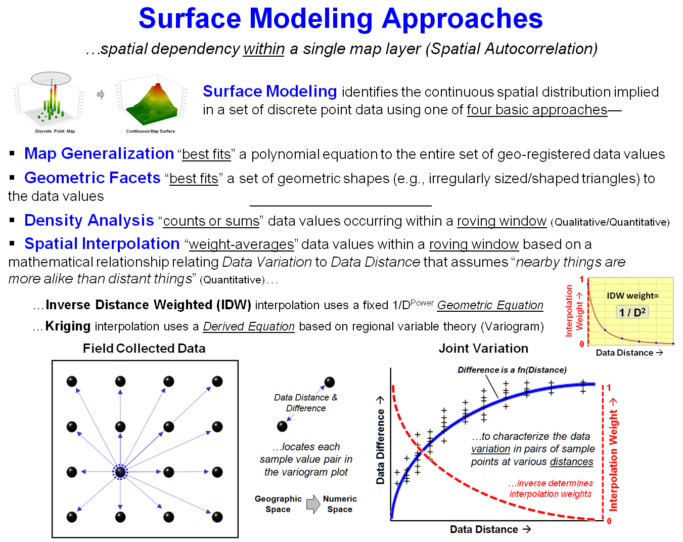
Figure 1. Spatial Statistics uses numerical
analysis to uncover spatial relationships and patterns.
Summaries among two or more discrete maps generate cross-tabular tables
that “count” the joint occurrence of all categorical combinations of the map
layers. For example, the coincidence of
steepness and cover maps might identify that there are 242 acres of forest
cover on extremely steep slopes (16 percent), a particularly hazardous wildfire
joint condition.
Map comparison and correlation techniques only apply to continuous
mapped data. Comparisons within a single
map surface involve normalization techniques.
For example, a Standard Normal Variable (SNV) map can be generated to
identify “how unusual” (above or below) each map location is compared to the
typical value in a project area.
Direct comparisons among continuous map surfaces include appropriate
statistical tests (e.g., F-test), difference maps and surface configuration
differences based on variations in surface slope and orientation at each grid
location.
Map correlations provide a foothold for advanced inferential spatial
statistics. Spatial autocorrelation
within a single map surface identifies the similarity among nearby values for
each grid location. It is most often
associated with surface modeling techniques that employ the assumption that
“nearby things are more alike than distant things”—high spatial
autocorrelation—for distance-based weight averaging of discrete point samples
to derive a continuous map surface.
Spatial correlation, on the other hand, identifies the degree of
geographic dependence among two or more map layers and is the foundation of
spatial data mining. For example, a map
surface of a bank’s existing concentration of home equity loans within a city
can be regressed against a map surface of home values. If a high level of spatial dependence exists,
the derived regression equation can be used on home value data for another
city. The resulting map surface of
estimated loan concentration proves useful in locating branch offices.
In practice, many geo-business applications utilize numerous
independent map layers including demographics, life style information and sales
records from credit card swipes in developing spatially consistent multivariate
models with very high R-squared values.
Like most things from ecology to economics to environmental
considerations, spatial expression of variable dependence echoes niche theory
with grid-based spatial statistics serving as a powerful tool for understanding
geographic patterns and relationships.
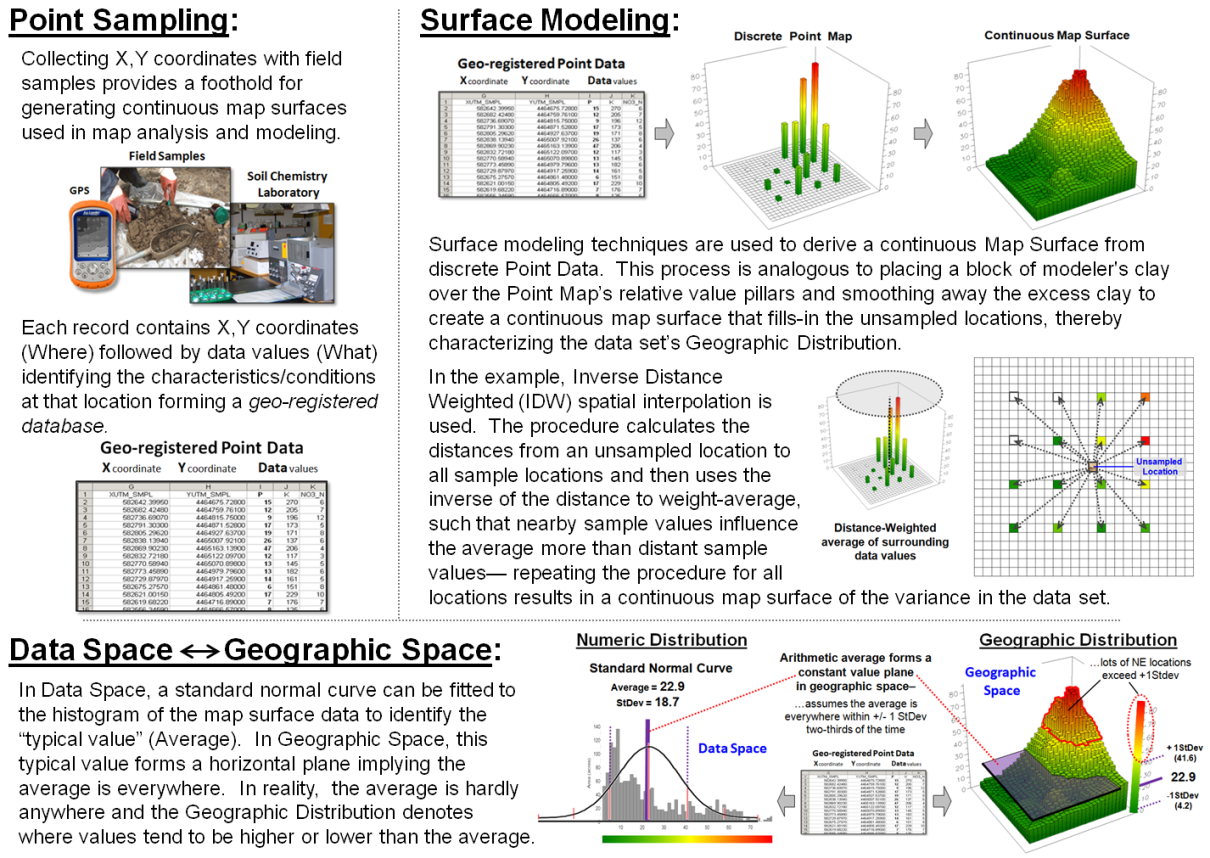
Figure 2. An example of Surface Modeling that derives a continuous map surface from set of
discrete point data.
Figure 2 describes an example of basic surface modeling and the linkage
between numeric space and geographic space representations using
environmentally-oriented mapped data.
Soil samples are collected and analyzed assuring that geographic
coordinates accompany the field samples.
The resulting discrete point map of the field soil chemistry data are spatially
interpolated into a continuous map surface characterizing the data set’s
geographic distribution.
The bottom portion of figure 2 depicts the linkage between Data Space
and Geographic Space representations of the mapped data. In data space, a standard normal curve is
fitted to the data as means to characterize its overall “typical value”
(Average= 22.9) and “typical dispersion” (StDev=
18.7) without regard for the data’s spatial distribution.
In geographic space, the Average forms a flat plane implying that this
value is assumed to be everywhere within +/- 1 Standard Deviation about
two-thirds of the time and offering no information about where values are
likely more or less than the typical value.
The fitted continuous map surface, on the other hand, details the
spatial variation inherent in the field collected samples.
Nonspatial statistics identifies the “central tendency” of the data,
whereas surface modeling maps the “spatial variation” of the data. Like a Rochart ink blot, the histogram and the map surface provide two different
perspectives. Clicking a histogram
pillar identifies all of the grid cells within that range; clicking on a grid
location identifies which histogram range contains it.
This direct linkage between the numerical and spatial characteristics
of mapped data provides the foundation for the spatial statistics operations
outlined in figure 3. The first four
classes of operations are fairly self-explanatory with the exception “Roving
Window” summaries. This technique first
identifies the grid values surrounding a location, then
mathematically/statistically summarizes the values, assigns the summary to that
location and then moves to the next location and repeats the process.
Another specialized use of roving windows is for Surface Modeling. As described in figure 2, inverse-distance
weighted spatial interpolation (IDW) is the weight-averaged of samples based on
their relative distances from the focal location. For qualitative data, the total number of occurrences
within a window reach can be summed for a density surface.
In figure 3 for example, a map identifying customer locations can be
summed to identify the total number of customers within a roving window to generate
a continuous map surface customer density.
In turn, the average and standard deviation can be used to identify
“pockets” of unusually high customer density.
Standard multivariate techniques using “data distance,” such as Maximum
Likelihood and Clustering, can be used to classify sets of map variables. Map Similarity, for example, can be used to
compare each map location’s pattern of values with a comparison location’s
pattern to create a continuous map surface of the relative degree of similarity
at each map location.
Statistical techniques, such as Regression, can be used to develop
mathematical functions between dependent and independent map variables. The difference between spatial and
non-spatial approaches is that the map variables are spatially consistent and
yield a prediction map that shows where high and low estimates are to be
expected.
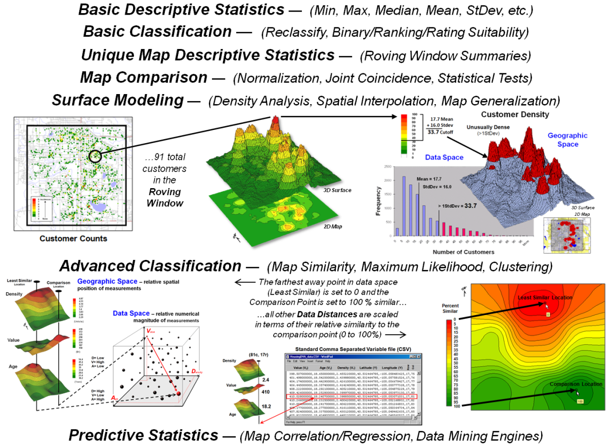
Figure 3. Classes of
Spatial Statistics operations.
The bottom line in spatial statistics (as well as spatial analysis) is
that the spatial character within and among map layers is taken into
account. The grid-based representation
of mapped data provides the consistent framework that needed for these
analyses. Each database record contains
geographic coordinates (X,Y= Where) and value fields
identifying the characteristics/conditions at that location (Vi=
What).
From this map-ematical view, traditional
math/stat procedures can be extended into geographic space. The paradigm shift from our paper map legacy
to “maps as data first, pictures later” propels us beyond mapping to map
analysis and modeling. In addition, it
defines a comprehensive and common spatialSTEM educational environment
that stimulates students with diverse backgrounds and interests to “think
analytically with maps” in solving complex problems.
_____________________________
Author’s
Notes: a table of URL links to
further readings on the grid-based map analysis/modeling concepts, terminology,
considerations and procedures described in this three-part series on
spatialSTEM is posted at www.innovativegis.com/basis/MapAnalysis/Topic30/sSTEM/sSTEMreading.htm.
The Spatial Key to Seeing the Big Picture
(GeoWorld,
September 2013)
Earlier discussion described the standard Latitude/Longitude grid as a
“Universal Spatial dB Key” that is comparable to the date/time tagging of
records in most database systems (“To Boldly Go Where No Map Has Gone
Before,” GeoWorld, October 2012).
With general availability of GPS coordinates on most data collection
devices, cameras, smartphones and tablets, earth position can be easily stamped
with each data record. Couple that with
geo-coding by street address and most data collected today has a triplet of
numbers indicating location (where), as well as characteristic/condition
(what)—XY and Value designating “where is what.”
Data flowing from a “spatially aware database” can be thought of as a
faucet spewing data that meets a query (figure 1). In turn, each value flows to the appropriate
grid cell based on its Lat/Lon tag. The
process can be conceptualized as the “what” attributes aligning within an
analysis frame (matrix of numbers) that characterizes the spatial
pattern/distribution inherent in a set of data.
While the long history of quantitative data analysis focused on the numerical
distribution of data, quantitative analysis of the spatial distribution
of geospatial data provides an new frontier for understanding spatial patterns
and relationships influencing most physical, biological, environmental,
economic, political and cultural systems.
The recognition, development and application of this fresh math/stat
paradigm (sort of a “map-ematics”) promises to
revolutionize how we extract and utilize information from field collected data
(see Author’s Note 1).
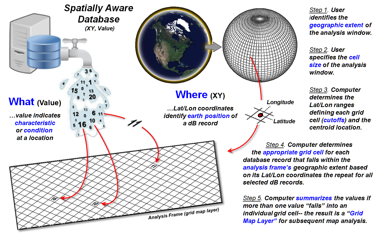
Figure 1. Steps in generating a grid map layer
from spatially tagged data.
Converting spatially tagged data into grid maps is outlined on the
right side of figure 1 as a five step process.
The user first identifies the “geographic extent” of an area of interest
by interactively dragging a box on a map or by entering Lat/Lon coordinates for
the boundary (Step 1).
An appropriate “cell size” for analysis is then entered as length of a
side of an individual grid cell (Step 2).
The smaller the cell size the higher the spatial resolution affording
greater detail in positioning but resulting in exponentially larger matrices
for storage. User judgment is applied to
balance the precision (correct placement), accuracy (correct characterization)
and storage/performance demands (see Author’s Note 2).
In Step 3, the computer divides the lengths of the NS and EW sides of
the project area extent by the cell size to determine the number of rows and
columns of a matrix (termed the Analysis Frame) used to store grid layer
information (map variables). This establishes
an algorithm for determining the Lat/Lon ranges defining each grid cell and its
centroid position. Considerations and
implications surrounding this technically tricky step (3D curved earth to 2D
flat matrix) are reserved for later discussion.
Based on the positioning algorithm’s calculations, each geo-tagged
value flowing from the database can be placed in the appropriate row/column
position in the analysis frame’s matrix (Step 4). The processing is repeated for all of the
selected dB records. If more than one
value “falls” into a grid cell the values are summarized on-the-fly (Step
5).
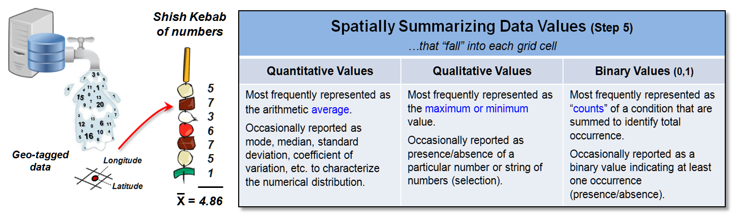
Figure 2. Summarizing
multiple data values falling in a single grid cell.
Figure 2 depicts the considerations surrounding the summary of multiple
data values sharing a single grid cell.
The condition can be conceptualized as a “shish kebab of numbers” that
needs to be reduced to an overall value that best typifies the actual
characteristic/condition at that location.
The data type of the numbers determines the summary techniques
available. Most often quantitative
values are averaged as shown in the figure but other statistical metrics can be
used depending on the application.
Qualitative values are typically assigned the maximum or minimum value
encountered in the string. Binary
values, such as crime occurrence, are usually summed to identify total count of
instances at each grid location.
The result of the five step procedure creates a grid map layer
identifying the “discrete” spatial pattern of the data that is analogous
to a histogram in non-spatial statistics.
In most applications, spatial interpolation or density analysis
techniques are used to derive a continuous grid map layer characterizing
the spatial distribution of the data which is analogous to fitting a standard
normal curve to a histogram (see Author’s Note 3). Once in this generalized form, most
traditional quantitative analysis techniques (plus some spatially unique
techniques) can be applied to investigate the spatial distribution, as well as
the numerical distribution of the data.
The muddling concerns in applying the Lat/Lon grid as a Universal
Spatial dB Key is in representing curved 3D earth positions as flat 2D cells of
a matrix. Figure 3 shows the reality of
the grid cell shape that morphs from squares to stretched rectangles to
elongated trapezoids with north/south movement away from the equator (see Author’s
Note 4).
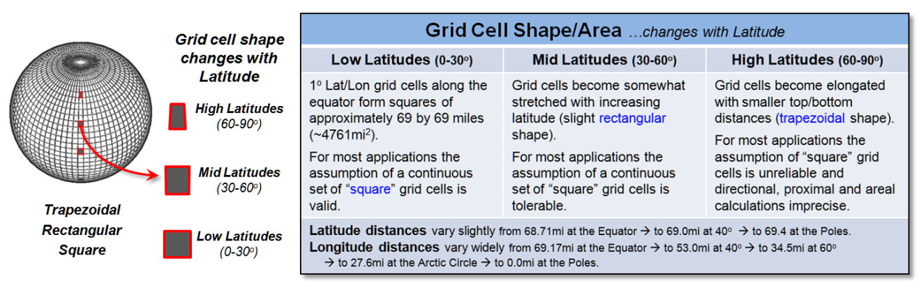
Figure 3. The area and shape of Lat/Lon
grid cells varies with increasing latitude.
Relatively small changes in the length of a degree of “latitude parallels”
occur because of polar flattening— earth is an oblique spheroid instead of a
perfect sphere due to centrifugal forces as the earth spins. However huge changes occur for “longitude
meridians” as the lines converge at the poles— a degree of longitude is widest
at the equator and gradually shrinks to zero at the poles.
The bottom line is that directly representing the Lat/Lon grid as a
two-dimensional matrix can be unreliable for large project areas at the higher
latitudes. However two caveats are in
play. One is that projection algorithms
can be applied on-the-fly to transform the curved 3D coordinates to a planar
representation and then back to lat/Lon.
The other is that for many applications involving relatively small
project areas at low or mid latitudes, the positional precision tolerable. The notion of “tolerable” precision is what
most differentiates “mapping” from “map analysis.” While neighbors and armies fight over inches
in the placement of borders, most data analysts are more accommodating and
satisfied knowing things are much higher (or lower) over there as compared to
here—a few inches or feet (or even miles in some cases) misplacement doesn’t
obscure the big picture of the spatial distribution and relationships.
_____________________________
Author’s Notes: 1) See, Topic 30, “A Math/Stat Framework for
Grid-based Map Analysis and Modeling;” 2) see Introduction, section 2,
“Determining Exactly Where Is What;” 3) see Topic 2, “Spatial Interpolation
Procedures and Assessment” and Topic 7, “Linking Data Space and Geographic
Space” in the online book Beyond Mapping III
posted at www.innovativegis.com/basis/. 4) For a detailed discussion of latitude and
longitude considerations see www.ncgia.ucsb.edu/giscc/units/u014/u014.html
in the NCGIA Core Curriculum in Geographic Information Science, by Anthony P. Kirvan and edited by Kenneth Foote.
Recasting Map Analysis Operations for General
Consumption
(GeoWorld,
February 2013)
Earlier discussions have suggested that there is “a
fundamental mathematical structure underlying grid-based map analysis and modeling
that aligns with traditional non-spatial quantitative data analysis” (see
Author’s Note 1). This conceptual
framework provides a common foothold for understanding, communicating and
teaching basic concepts, procedures and considerations in spatial reasoning and
analysis resonating with both GIS and non-GIS communities—a SpatialSTEM schema—that
can be applied to any grid-based map analysis system (see Author’s Note
2).
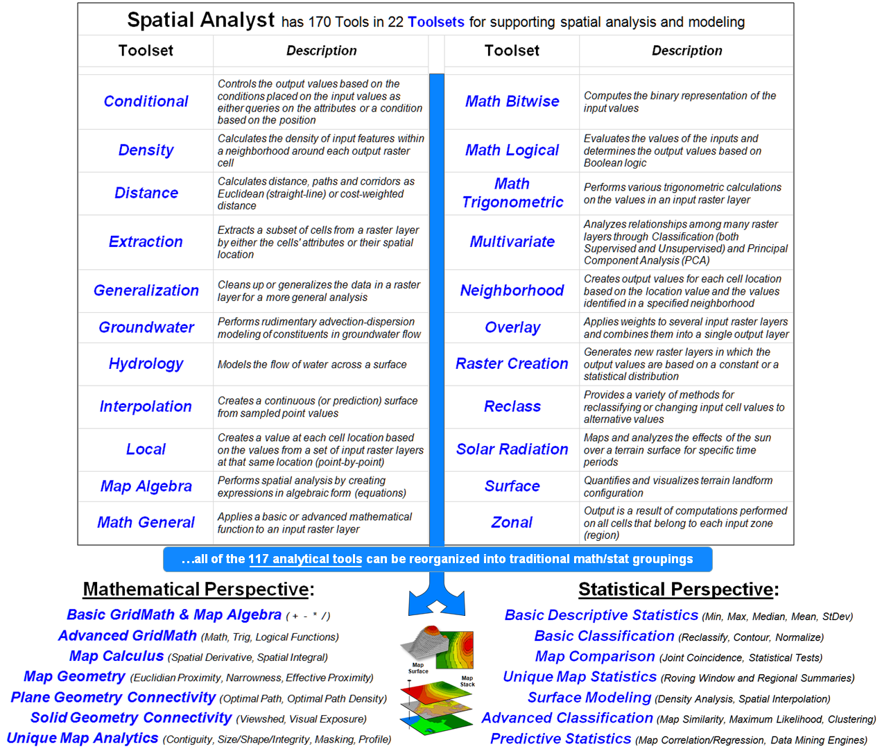
Figure 1. Grid-based map analysis
operations in any GIS system, such as Spatial Analyst, can be reorganized into
commonly understood classes of traditional quantitative data analysis.
For example, the top portion of figure 1 identifies the 22 map analysis
“toolsets” containing over 170 individual “tools” in the Spatial Analyst module
(ArcGIS by Esri). The organization of
the classes of operations involves a mixture of—
-
Traditional math/stat procedures (Conditional, Map Algebra, Math
General, Math Bitwise, Math Logical, Math Trigonometric, Multivariate, Reclass);
-
Extensions of traditional math/stat procedures (Distance,
Interpolation, Surface);
-
Unique map analysis procedures (Density, Local, Neighborhood,
Overlay, Zonal);
-
Application-specific procedures (Groundwater, Hydrology, Solar
Radiation); and
-
Housekeeping tasks (Extraction, Generalization, Raster
Creation).
In large part, this toolset structuring is the result of the module’s
development over-time responding to “business case” demands by clients instead
of a comprehensive conceptual organization.
In contrast, Tomlin’s “Local, Focal, Zonal and Global” classes
characterize the analytical operations on how the input data is obtained for
processing, while my earlier groupings of “Reclassify, Overlay, Distance,
Neighbors and Statistical” reflect the characteristics of the mapped data
generated by the processing.
However, all three of these GIS-based schemas are foreign and confusing
to the vast majority of potential map analysis users (all STEM disciplines) as
they do not align with their traditional quantitative data analysis
experiences. This conceptual disconnect
keeps GIS on the sidelines of the much larger quantitative analysis communities
and reinforces the idea that GIS is a “technical tool” (mapping and geoquery)
not a full-fledged “analytical tool” (spatial analysis and statistics).
The bottom portion of figure 1 identifies the two broad categories of
traditional data analysis— Mathematics and Statistics—broken into seven major
groupings that resonate with non-GIS communities. All of Spatial Analysts’ 117 analytical
operations (the other 53 are “reporting/housekeeping”) can be reorganized into
the commonly recognized quantitative analysis categories.
Figures 2 and 3 at the end of this section
show my initial attempts at the reorganization (see Author’s Note 3).
The bottom line is that the SpatialSTEM framework recasts map analysis
concepts and procedures into a more generally understood organization. Within this general schema, map analysis is
recognized as a set of natural extensions to familiar non-spatial math/stat
operations. For example—
-
A high school math teacher might follow a discussion of the
Pythagorean Theorem with “…but what if there is an impassible barrier between
the two points? The distance is no
longer a straight line but some sort of a ‘bendy-twisty’ route around the
barrier. How would you calculate the
not-necessarily-straight distance? The
‘Splash Algorithm’ does that by…” (you know the rest
of the story).
-
Or a statistics instructor might follow a lecture on the
derivation of the Standard Normal Curve for characterizing the ‘numerical
distribution’ of a data set with “…but what about the ‘spatial distribution’ of
the data? Is data always uniform or
randomly distributed in geographic space?
How could you characterize/visualize the spatial distribution? ‘Spatial Interpolation’ does that by…” (you know the rest of the story).
-
Or an environmental science teacher might follow a lecture on
the use of riparian buffers with “…but are all ‘buffer-feet the same’? What about the slope of the surrounding
terrain? …and the type of soil? …and the density of vegetation? Wouldn’t an area along a stream that is steep
with an unstable soil and minimal vegetation require a much larger setback than
an area that is flat with stable soils and dense vegetation? How could you create a variable-width buffer
around streams that considers the intervening erosion conditions? A simple ‘sediment loading model does that
by…” (you know the rest of the story).
-
Or a crop scientist who historically calculated the increase
(decrease) in yield over a previous year for a new genetic variety as the
percent change in the total “weigh-wagon” records for an entire trial
field. But with GPS-enabled yield maps
that automatically collect on-the-fly yield measurements as a harvester moves
through a field, a detailed map of the percent change can be generated by spatially
evaluating the standard algebraic equation by… (you
know the rest of the story).
-
Or a sales manager can use ‘address geo-coding’ to sprinkle
sales data onto a grid map and then compute ‘roving window’ totals to generate
a sales density surface showing where sales are high (or low) throughout each
of several sales territories. The map
analysis can be extended to calculate areas of unusually high (or low) sales by
identifying locations that are more than one standard deviation above (or
below) the average sales density… (you know the rest
of the story).
Dovetailing map analysis with traditional quantitative analysis
thinking moves GIS from a “specialty discipline down the hall and to the right”
for mapping and geoquery, to an integrated and active role in the spatial
reasoning needed by tomorrow’s scientists, technologists, decision-makers and
other professionals in solving increasing complex and knurly real-world
problems. From this perspective,
“thinking with maps” becomes a true fabric of society thus fulfilling GIS’s
mega-technology promise.
…the following two listings
cross-reference Spatial Analysis tools in ArcGIS software
by Esri to commonly recognized
quantitative math/stat analysis categories—
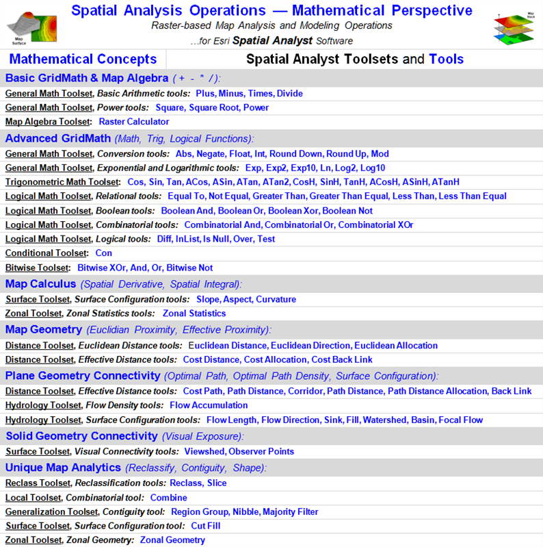
Figure 2. Reorganization
of Spatial Analyst’s analytical “tools” into traditional mathematical
categories.
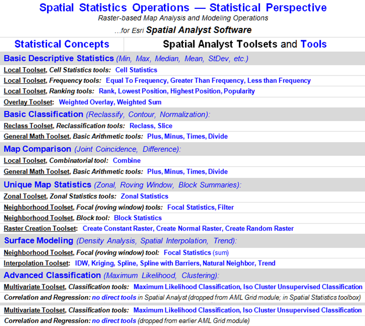
Figure 3. Reorganization
of Spatial Analyst’s analytical “tools” into traditional statistical
categories.
_____________________________
Author’s Note: 1) see the Chronological Listing of Beyond Mapping
columns posted at www.innovativegis.com/basis/MapAnalysis/ChronList/ChronologicalListing.htm;
2) for numerous links to papers, PowerPoint slide sets and other materials
describing the SpatialSTEM framework, see www.innovativegis.com/Basis/Courses/SpatialSTEM/;
3) at the same SpatialSTEM posting, see the white paper entitled “Math/Stat
Classification of Spatial Analysis and Spatial Statistics Tools (Spatial
Analyst by Esri)” more detailed description of the recasting of Spatial
Analyst’s operations by traditional non-spatial mathematics and statistics
categories.
(Back to the Table of Contents)