|
Beyond
Mapping III Topic 8
– Spatial Modeling Example (Further Reading) |
Map Analysis book |
(Extending
Optimal Path Analysis)
’Straightening’
Conversions Improve Optimal Paths — discusses a procedure for spatially
responsive straightening of optimal paths (November 2004)
Use
LCP Procedures to Center Optimal Paths — discusses a procedure for
eliminating “zig-zags” in areas of minimal siting preference (March 2006)
Connect
All the Dots to Find Optimal Paths — describes a procedure for
determining an optimal path network from a dispersed set of end points (September 2005)
(Understanding
Accumulation Surfaces)
Building
Accumulation Surfaces — reviews how proximity analysis and
effective distance is used to construct accumulation surfaces (October 1997)
Analyzing
Accumulation Surfaces — describes how two surfaces can be
analyzed to determine the relative travel-time advantages (November 1997)
Determining
Optimal Path Corridors — describes a technique for
determining the set of nth best paths between two points (December 1997)
Analyzing
Stepped Accumulation Surfaces — describes a technique for
forcing an optimal path through a series of points (January 1998)
<Click here> for a printer-friendly version of this topic (.pdf).
(Back
to the Table of Contents)
______________________________
(Extending Optimal Path Analysis)
’Straightening’ Conversions Improve Optimal Paths
(GeoWorld, November
2004)
Previous discussions (July through August 2003 BM columns) have
addressed the basics of optimal path routing.
The basic Least Cost Path (LPC) method described consists of three
basic steps: Discrete Cost Map, Accumulated Cost Surface and Optimal
Route (see Author’s Notes). In
addition, an optional fourth step to derive an Optimal Corridor can be
performed to indicate routing sensitivity throughout a project area.
Key to optimal path analysis is the discrete cost map that establishes
the relative “goodness” for locating a route through any grid cell in a project
area. However, the traditional
For example, the same optimal solution is generated for both low and
high priced pipe in constructing a pipeline.
In the case of higher priced pipe, a straighter route can save millions
of dollars. What is needed is a modified
Simple geometry-based techniques of line smoothing, such as spline
function fitting, are inappropriate as they fail to consider intervening
conditions and can result in the route being adjusted into unsuitable locations
as it is “smoothed.” The following
discussion describes a robust technique for “straightening” an optimal path
that works within the
The approach modifies the discrete cost map by making disproportional
increases to the lower map values. This
has the effect of straightening the characteristic minor swings in routing in
the more favorable areas (low values) while continuing to avoid unsuitable
areas.
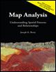
Figure 1. The
The left side of figure 1 graphically depicts the modified
The general conversion equation based on an anchored straight line is—
Y = i + (( 9 – i ) / 9 ) * X
…and can be extended to the
Adj_Cost_Map = i + (( 9 – i ) / 9 ) * Cost_Map
…where all of the values on the discrete cost map are converted. The adjusted cost map is used to derive an
accumulated cost surface from the starting location, that in turn is used to
derive the optimal path from the ending location.
Figure 2 shows several examples of applying the
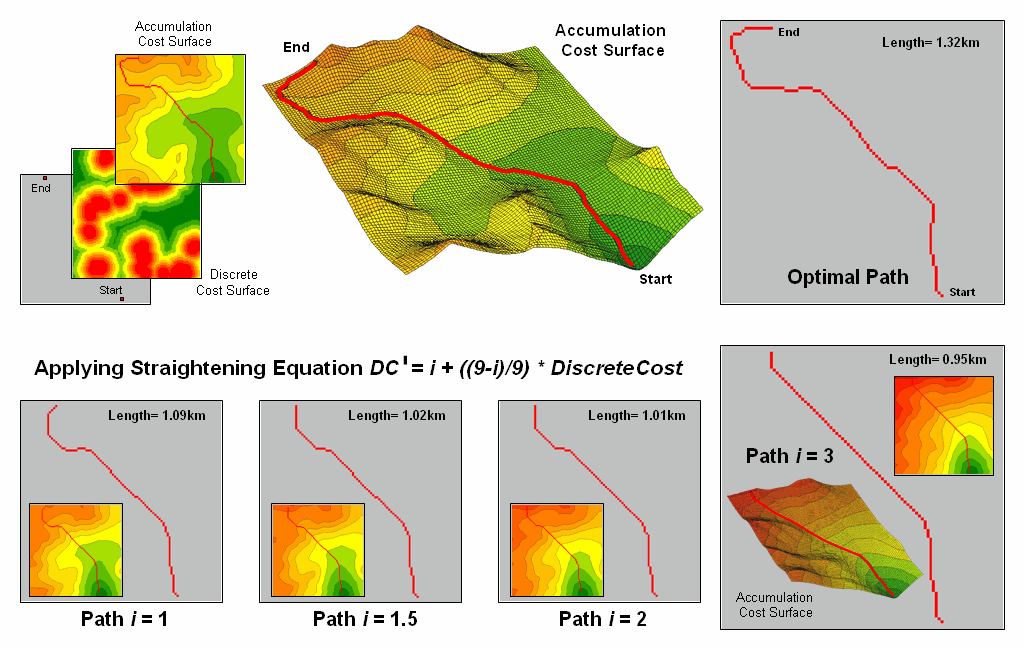
Figure 2. Examples of Applying the
The lower portion of the figure shows several straightened optimal
paths. They were derived by applying the
conversion equation to the discrete cost values, then completing the
Also note that the length of the route is progressively shorter for the
straightened optimal paths. This
information can be used to estimate pipe cost savings ((1.32 – 0.95) / 1.32) *
100 = 28% savings for Path 3).
Decision-makers can balance the benefits of the savings in materials
with the costs of traversing less-optimal conditions along the straightened
route as compared to the non-straighten optimal path.
The traditional unadjusted optimal path is best considering only
landscape/terrain conditions, whereas the adjusted path also favors
“straightness” wherever possible. In many
applications, that’s an improvement on an optimal path (as well as an
oxymoron).
______________________________
Author’s Note: see www.innovativegis.com/basis/present/Oil&Gas_04/
, A Web-based Application for Identifying and Evaluating Alternative Pipeline
Routes and Corridors, Berry, J.K., M.D. King and C. Lopez, for a paper
describing the basic
Use LCP Procedures to Center Optimal Paths
(GeoWorld, March
2006)
Earlier sections have dealt with basic Least Cost Path (
For example, routing pipelines involves identifying the optimal path
between two points considering an overall cost surface of the relative siting
preferences throughout a project area.
This established procedure works well in areas where there are
considerable differences in siting preferences but generates a “zig-zag” route
in areas with minimal differences. The
failure to identify straight routes under these conditions is inherent in the iterative
(wave-like) grid-based distance measurement analysis considering only
orthogonal and diagonal movements to adjacent cells.
The left side of Figure 1 shows the Optimal Corridor for a proposed
route. The central (blue) zone
identifies the “valley bottom” of the Total Accumulation Surface that contains
the optimal path. The middle zone
(green) and outer zone (yellow) identify areas that contain less optimal but
still plausible solutions.
Figure 1. “Flat areas” on the
valley bottom of the Total Accumulation Surface (blue) are the result of
artificial differences in optimal paths induced by grid-based distance
measurement restriction to orthogonal and diagonal movements.
The right side of the figure shows what causes the flat areas. The white route identifies the common
locations for the optimal paths generated for both ways (Start-to-End and
End-to-Start paths). These locations
identify the true optimal path in areas with ample preference guidance. However in areas with constant cost surface
values, the grid-based procedure seeks orthogonal and diagonal movements
instead of a true bisecting line. For
the area in the lower-right portion of the project area, the Start to End path
(bright green upper route) shifts over and diagonally down. In the same area, the End to Start path
(light blue lower route) shifts over and diagonally up.
The true optimal path traversing this area of minimal difference in
siting preferences is a line splitting the difference between the two
directional routes. Figure 2 depicts the
steps for delineating a centered route through these areas. The first step generates a Total Accumulation
Surface in the basic
This map is normally used to identify optimal path corridors, however
in this instance it is used to isolate the flat areas in need of
centering. A binary map of the flat
areas is created in step 2 by reclassifying areas to zero that are from the
minimum value on the surface to the minimum value + .707. The .707 value is determined as one-half a
diagonal grid space movement of 1.414 cells—the “zig-zag distance” causing the
flat areas.
The third step determines the interior proximities for the flat areas,
with larger values indicating the center between opposing edges. The proximity values then are converted to
adjustment weights from nearly zero to 1.0 (step 4). This process involves inverting the proximity
values then normalizing to the appropriate range by using the equation—
Weight
= ((0.00 – ProxValue) + maxProxValue) / (maxProxValue + .01)
The result is a map with the value 1.0 assigned to all locations that
do not need centering and increasing smaller fractional weights for areas
requiring centering. This map then is
multiplied by the original cost surface (step 5) with effect of lowering the
cost values where centering is needed.
The result is analogous to cutting a groove in the cost surface for the
flat areas that forces the optimal path through the centered groove (step 6).
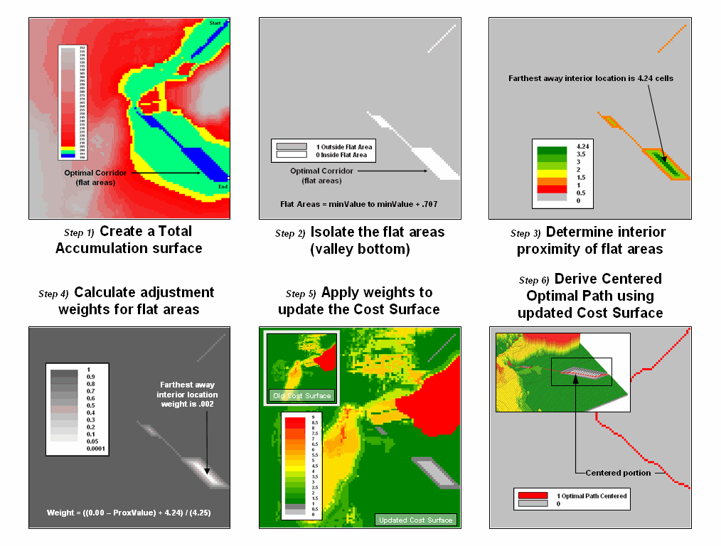
Figure 2. Procedural steps for
centering an optimal path in areas with minimal differences in siting
preference.
Figure 3 shows the results of the centering procedure. The red line bisects the problem areas and
eliminates the direction dependent “zig-zags” of the basic
In practice, an automated procedure for eliminating zig-zags might not
be needed as the optimal route and corridor identified are treated as a
Strategic Phase solution for comparing relative advantages of alternative
routes. A set of viable alternative
routes is further analyzed during a Design Phase with a siting team considering
additional, more detailed information within the alternative route
corridors. During this phase, the
zig-zag portions of the route are manually centered by the team—the art in the
art and science of
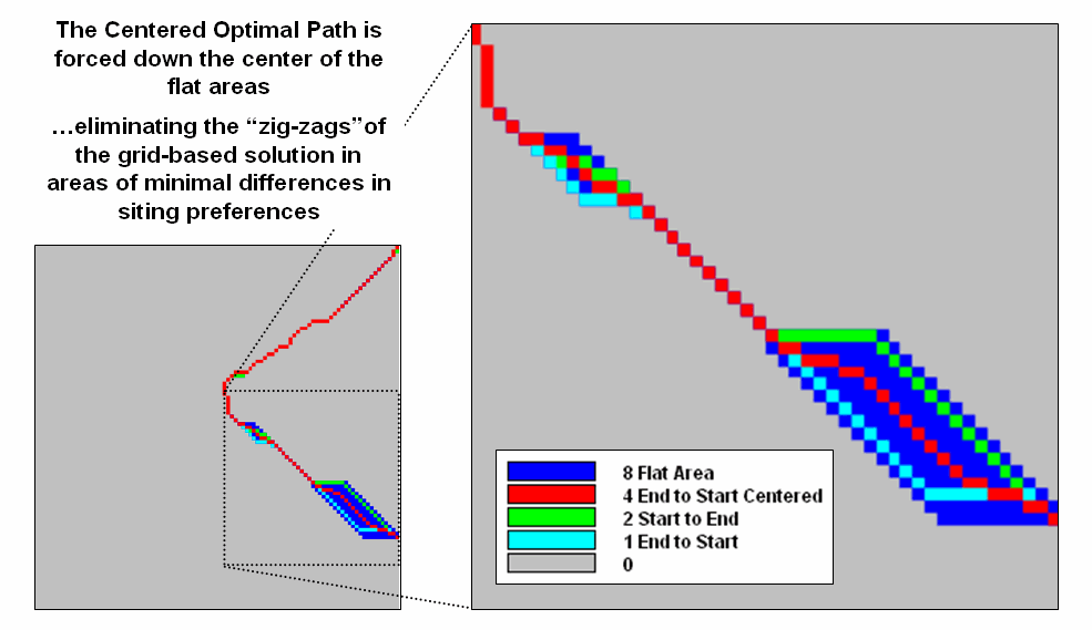
Figure 3. Comparison of
directional optimal paths and the centered optimal path.
Connect All the Dots to Find Optimal Paths
(GeoWorld,
September 2005)
Effective Distance forms the foundation for generating optimal
paths. As discussed in the previous
sections, the “Least Cost Path” method for determining the optimal route of a
linear feature is a well-established grid-based
The derivation of the Accumulated Cost Surface is the critical
step. It involves calculating the
effective distance from a starting location to all other locations considering
the “relative preference” for favoring or avoiding certain landscape
conditions.
For example, the left side of figure 1 shows a set individual cost maps
for establishing a gathering network of pipelines for a natural gas field. The thinking is that routing should—
1) avoid
areas within or near sensitive areas,
2) avoid
areas that are far from roads, and
3) avoid
areas of steep terrain, and 4) avoid areas of unsuitable soils.
These considerations first are calibrated to a common preference scale
(0= no-go, 1= favor through 9= avoid) and then averaged for an overall Discrete
Cost Map (favor green, avoid red and can’t cross black).
In turn, the discrete cost map is used to calculate effective distance
(minimal cost) from the collection point to all accessible locations in the
project area. The result is the
Accumulated Cost Surface shown in 2D and 3D on the right side of figure 1. Note that the surface forms a bowl with the
collection point at the bottom, increasing total cost forming the incline
(green to red) and the inaccessible locations forming pillars (black).
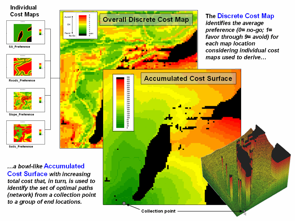
Figure 1. Relative preferences are
used to identify the minimal overall cost of constructing a route from a
collection point to all accessible locations in a project area.
Normally, a single end point is identified, positioned on the
accumulated surface and the steepest downhill path determined to delineate the
optimal route between the starting and end points. However in the case of a gathering network, a
set of dispersed end points (individual wells) needs to be considered. So how does the computer simultaneously mull
over bunches of points to identify the set of Optimal Paths that converge on
the collection point?
Actually, the process is quite simple.
In an iterative fashion, the optimal path is identified for each of the
wells. What is different is the use of a
summary grid that counts the number of paths passing through each map
location. The map in figure 2 shows the
result where red dots identify the individual wells, blue paths individual
feeder lines and cooler to warmer tones an increasing number of commonly served
wells.
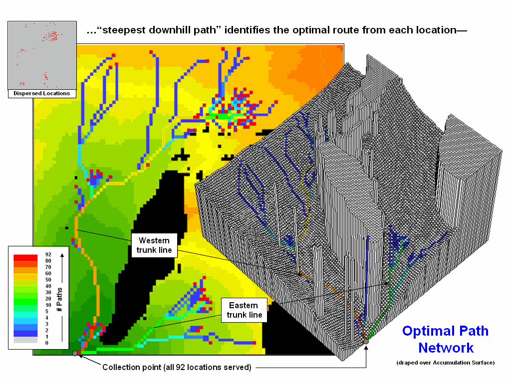
Figure 2. Optimal path density
identifies the number of routes passing through each map location.
The green, yellow and red portions of the network identify trunk lines
that service numerous end points (>10 wells). The collection point services all 92 wells
(77 from the western trunk line and 15 from the eastern trunk line).
Figure 3 shows the gathering network superimposed on the optimal
corridors for the western and eastern trunk lines. The corridors indicate the spatial
sensitivity for sighting the two trunk lines— placement outside these areas
results in considerable increase in routing costs.
In the example, a pressurized network is assumed. However, a gravity-feed analysis could be
performed by analyzing a terrain surface (relative elevation) and hydraulic
flows. The process is analogous to
delineating watersheds then determining the optimal network trunk lines within
each area.
Another extension would be to minimize the length of the feeder
lines. For example, the three lines in
the upper-left corner might be connected sooner to minimize pipeline materials
costs. There are a couple of ways to
bring this into the analysis— 1) re-run the model using the trunk line as the
starting location, and/or 2) use a straightening factor as discussed in the
previous section.
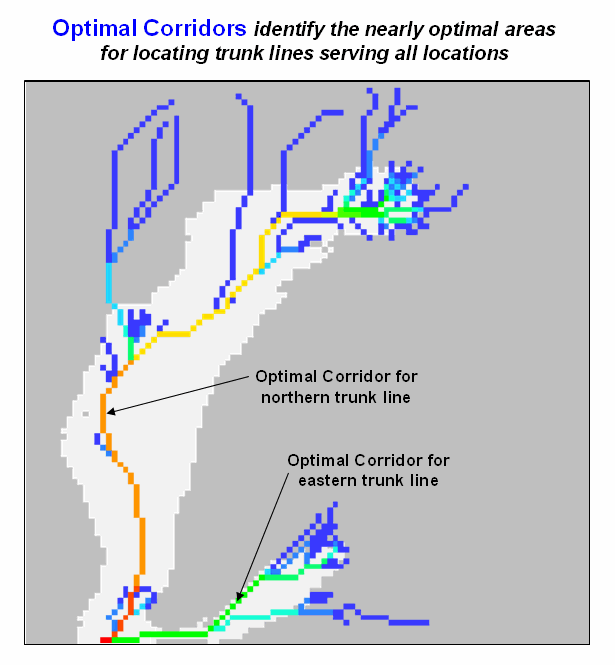
Figure 3. The
optimal corridors for routes serving numerous end points indicate the spatial
sensitivity in siting trunk lines.
The ability to identify the number of optimal paths from a set of
dispersed end points provides the foothold for deriving an optimal feeder line
network. It also validates that modern
map analysis capabilities takes us well-beyond traditional mapping to entirely
new concepts, techniques and paradigms spawned by the digital map revolution.
(Understanding Accumulation
Surfaces)
Building
Accumulation Surfaces
(GeoWorld, October
1997)
“You can’t get there from here,” is often the flippant response when
you ask directions. In many cases it is
a perfectly valid answer, as movement in geographic space is rarely as straight
forward as a straightedge. Often there
are several possible contorted paths that twist and turn in route to a
destination. However, from the
perspective of a ruler there is only one— the “shortest, straight line
connecting two points.” Several Beyond
Mapping columns (see Author’s Note) have addressed the concepts and procedures
behind
Before we get too far, a quick review might be prudent. Recall that there are primarily two ways to
represent distance in a
c2
= a2 + b2
from the brow-beating you received about right triangles in high school
geometry. The
The splash technique tracking simple proximity is a bit less familiar, but
conceptually easy. Imagine what happens to a still pond when you toss in a
rock— splash, then one ripple away, then another, and another, until there’s a
whole set of concentric rings about the starting point. If the conditions are the same throughout the
pond, the effect is similar to nailing a ruler at the starting point and
spinning it, while scribing the set of circles formed by dragging the ruler’s tic
marks. In a raster
Now imagine tossing a handful of rocks— splash, one ripple, two ripple, three
ripple, and more radiate out from each of the starting points. When two wave-fronts meet, they stop, with
the point of interference identifying the halfway location between starting
points. The same holds true if you toss
in a set of sticks or pieces of plywood, with the ripple patterns conforming to
the irregular shapes of the objects. The
end result of all the simulated splashing and crashing in a
Inset (a) in figure 1 is a 3-D plot of a simple proximity surface
radiating from a single point. The
lowest point on the surface contains the value 0 denoting it is “0 grid spaces
away” from the start. Note that the
surface is shaped like a bowl with increasing values (1 away, 2 away,
etc.). The farthest location is in the
upper right corner at a distance of 60 grid spaces * 100 meters/grid space =
6000 meters. The slight depressions
along the orthogonal and diagonal are a result of the slight directional
variations in distances computed by the “splash” algorithm.
But continuous, straight line movement forming a perfect proximity bowl
is rarely the case in the real world.
Effective proximity respects movement around and through barriers— not
“as the crow flies,” but as the crow might walk. Suppose there’s a lake in the way. Inset (b) identifies the absolute barrier
itself as being infinitely far away (fear/reality of drowning). It assigns a value of 69 grid spaces to the
farthest accessible location, indicating that the distance is a 900 meters farther
as a result of going around the lake.
The set of all map values indicate the “shortest, but not necessarily
straight” distances between the starting point and all of the other locations.
Figure 1. Accumulation surfaces
showing the effects of relative and absolute barriers in mapping proximity.
However, in winter the lake freezes and can be crossed, though at a
much slower pace on the slippery ice. It
represents a relative barrier that impedes movement, but doesn’t totally
restrict movement. Inset (c) shows the
accumulation surface assuming you walk 5 times slower on the ice. The results show that it’s still 6900 meters
to the opposite corner by going around the lake. However, if you gingerly trek to the center
of the lake, it is equivalent to traveling 8300 meters on open land.
Previous Beyond Mapping columns described how the computer finds the “steepest,
downhill path” along an accumulation surface to locate the “not necessarily
straight” optimal path. It’s analogous
to a rain drop’s route along the surface, which effectively retraces the wave
front that got there first. In fact, the
rain drop paths from all locations identify the “shortest, but not necessarily
straight set of lines connecting the origin to everywhere.” Information you with a ruler, or Pythagoras
with a calculator, could never derive.
But it’s chicken-feed compared to what insights you get by analyzing the
surfaces themselves— as you will see in the next section.
_____________________
Author’s Note: see
Analyzing Accumulation Surfaces
(GeoWorld,
November 1997)
The previous section described the nature of accumulation surfaces and
how they are built. Recall that the
“splash” algorithm measures distance from a starting location like waves that
spread out when a rock is tossed into a pond.
The result is a 3-dimensional surface with increasing distance reflected
by the increasing Z values stored in a matrix of grid cells. If absolute and relative barriers to movement
are introduced, these surfaces form unique shapes with ridges and peaks similar
to terrain surfaces.
However, unlike terrain surfaces, accumulation surfaces are always increasing
(no “false-bottoms”) from point, line and areal features designated as starting
locations. Areas with absolute barriers
are identified as infinitely far away and form sheer walls on an accumulation
surface. Relative barriers form hills
and ridges as they identify areas that are passable, but at an increased “cost”
(e.g., more time) per grid space. The
valleys emanating from the starting locations locate corridors of minimal
resistance to movement along the accumulation surface.
Figure 1. The difference between
two proximity surfaces identifies the relative geographic advantage between two
locations.
For example, the two surfaces on the extreme left of figure 1
characterize movement from opposing corners through the horseshoe-shaped
relative barrier described in the previous section. The proximity from Start1 generally increases
from left to right, while the increase from Start2 is in the opposite
direction. Both surfaces show an abrupt
increase when the relative barrier is encountered, however the shape of the
resulting “hill” is different due to the different directions of the distance
waves and the shape of the barrier.
Since the horseshoe ends of the barrier face Start1, the waves easily move into
the center before interacting with the increased impedance of the barrier. The formation of a ridge indicates that some
of the waves moved around the barrier, then penetrated the barrier from the
back side. Any location along the ridge
is equally distant from the start by moving to either side of hill.
The locations on the back side of the ridge, however, are optimally
connected to Start1 by moving down the hill to the right and around the
barrier… a counter-intuitive move.
Neither ruler nor Pythagoras’ Theorem suggest that you must initially
move away from Start1 to begin the optimal route connecting the location to
Start1. That’s because they simply
assume that all movement is in a straight line connecting two points— an
extremely limiting assumption in the real world of complex barriers.
The vertical line intersecting both surfaces identifies a map location that is
63 grid spaces from Start1 and only 5 from Statrt2. Since these “shortest, but not necessarily
straight” distances are stored at the same column, row position in the two
proximity matrices, they can be easily retrieved and their difference computed
(63 - 5 = 58). If this is done for all
locations, a difference surface (S1-S2 Surface inset in the middle of the
figure) is generated identifying the relative advantage between Start1 and
Start2 access for all locations throughout the project area.
The “0” line identifies locations that are equally distant between the two
starting locations. It’s similar to the
“perpendicular bisector” you might remember from high school geometry, except
it is bent and twisted reflecting the effect of the intervening barrier on
actual movement. The sign of the
difference indicates who has the advantage— negative values identify locations
where Start1 has an advantage; positive values indicate a Start2
advantage. The magnitude of the value
identifies the strength of the advantage.
The two surfaces on the right isolate the relative advantages for both
starting locations. Similar advantage
surfaces can be derived for additional starting locations, keeping in mind that
the “starters” can be any combination of point, line or areal features.
In the example, a +58 denotes a location with a strong advantage for Start2
access… it would be stupid to trek all the way to Start1. If you were a thirsty animal (or pub patron),
why would you travel the extra distance?
The liquid libations would have to be a lot better, or the ambiance and
other thirsty organisms much more to your liking. If that were the case, then the relative
attractiveness of starter locations can be incorporated into the derivation of
the accumulation surfaces (termed “gravity” modeling).
Accumulation surface analysis provides valuable information for a wide array of
applications. Natural resource managers
use the technique to identify “home ranges” and “corridors of movement” based
on the arrangement of landscape features.
Instead assuming a simple distance of “within a two mile radius” of an
animal’s burrow, an effective distance home range based on absolute (e.g.,
river) and relative (e.g., cover type preferences) barriers can modeled.
Similarly, a retail market analyst can model the “home range” of a particular
breed of shopper by characterizing the road network (e.g., speed limit) and
ancillary attractions (e.g., areas of interest). Or in-store shopper habitat can be modeled
using the aisles like roads and department fixtures as attractions; even
“blue-light specials” could be modeled as dynamic features in a real time
system. Traffic flows, whether in-store,
across town or in the wild are similar beasts from a
__________________________________
Author’s Note: for “hands-on” experience in deriving
and analyzing accumulation surfaces, see exercises TMAP2, TUTOR5, TUTOR6 and
TU-
Determining
Optimal Path Corridors
(GeoWorld,
December 1997)
The
first section in this series described the construction and fundamental nature
of accumulation surfaces. The second
section discussed an analysis procedure for mapping relative geographic
advantage that involved subtracting two surfaces. This time we will investigate the
interpretation of slope and aspect of an accumulation surface and what
information is derived if we add the surfaces.
Figure 1. The sum of two proximity
surfaces identifies the optimal path between two locations as the lowest
values, while increasing values identify the “opportunity cost” of forcing a
path through any location.
Recall
that as distance increases from a location(s) the values can be plotted as a
3-dimensional surface, like those shown in the left portion of figure 1. The lowest point on the surface identifies
the starting location(s) as zero units away from itself. All other locations contain increasing
distance values forming the characteristic “bowl-shape” of an accumulation
surface.
Effective
distance (as opposed to “simple,” straight-line distance) can be derived by
introducing absolute and relative barriers to movement. The “hill” in the Starter1 and Starter2
proximity surfaces reflect the increased impedance of a horseshoe-shaped
barrier in the center of the map area.
Each grid space on a friction map is coded with the “relative cost” of
traversing that location. Note that the
increased impedance is translated into the steeper slopes for the barrier
area. Therefore a slope map of an
accumulation surface unmasks the relative ease of optimal travel through each
grid space.
The notion of “optimal movement” embedded in an accumulation surface is
important. The “splash” algorithm used
to build the surface considers movement from the eight surrounding cells to
each location. The accumulated distance
and the relative impedance for each of the eight potential “steps” is
evaluated. The least costly step, in
terms of total movement, is assigned.
Therefore an aspect map of an accumulation surface unmasks the direction
of optimal movement through each grid space.
That’s a lot of spatially-specific information— the rate and direction of
optimal movement throughout a map area.
It allows us to relax the assumption that “everything moves in a
straight line and with equal impedance.”
In fact, things rarely move as simply as they respond to the complex
patterns of absolute and relative barriers existing in the real world. Slope and aspect maps of an accumulation
surface allow us to track the conditions of that complex movement at each map
location.
As described in the first article, the optimal path from any location to the
origin is identified as the steepest downhill route over the surface. In the second article, we found that
subtracting two accumulation surfaces located the bisecting line between the
origins as 0 (equidistant). The sign of
the distance value on the difference map indicated which origin was closer, and
its magnitude indicated how much closer.
For
example, a wildfire response model might generate a proximity map for two fire
stations considering both on and off-road movement. Subtracting the maps locates the effective
dividing line between the two stations.
In retail marketing, the halfway line is extended into a broad band
indicating a “combat zone” for customers.
Areas outside the band have distinct proximity advantages, while the
real battles are waged in the combat zone where there the differences are
marginal.
If subtracting accumulation surfaces creates useful information, what do you
think happens when you add them? The
surface in the center of the figure is a summation surface for the example
data. The highlighted location is 63
from Start1 and 5 from Start2, therefore it is a total of 68 units away from
both. In other words, the best path
connecting the two origins which passes through that location has a total
length of 68. In fact, the values on the
summation surface identify the length of the “best” path forced through any
given map location.
The optimal path between the two locations (identified by the line in both the
2-D and 3-D views) contains the set of locations having the lowest values (a
valley connecting the origins). The
saw-toothed appearance of the optimal path is an artifact of arithmetic
rounding, the nature of the splash algorithm and minimal friction outside the
barrier in the center. Values above the
valley floor indicate the length of the best, but sub-optimal paths forced
through any location.
The difference between the lowest value on the summation surface and the value
at any other location identifies the “opportunity cost” of forcing a route
through that location. The 2-D display
shows fixed intervals of increasing opportunity cost— you would be crazy to
force a route through the darker tones (a mountain of opportunity cost). Next time we will look at constructing a
“stepped accumulation surface” which enables you to determine the optimal path
connecting a series of predetermined stops along the way. As a sneak preview, it involves minimizing
successive accumulation surfaces… whew!
Analyzing
Stepped Accumulation Surfaces
(GeoWorld, January
1998)
Hopefully you have survived the last three sections on accumulation
surfaces. The discussion has covered the
fundamental nature of accumulation surfaces (increasing distance waves),
procedures for determining relative geographic advantage (subtract), ways to
uncover direction and speed of optimal movement (slope and aspect), and a
technique for determining the corridor of optimal movement (add). If that wasn’t enough, now we get to extend
the discussion to a “stepped accumulation surface” and “optimal path zones.”
Figure 25.4. Stepped Accumulation
Surface. Proximity from the first point is calculated (shaded) until the second
point is reached, then proximity from that point is calculated (non-shaded)
forming the next tier; the individual optimal paths along each of the stepped
proximity surfaces forms the overall optimal route.
Suppose you know several places you would like to visit, but don’t have
a particular route in mind. If you know
the order you would like to visit them, then a directed stepped accumulation
surface is for you. Simply generate an
effective proximity surface from the first location like those discussed in the
previous articles— splash, one ripple, two ripple, three ripple and more
radiate out from your starting point.
The familiar bowl of proximity identifies the effective distance to all
other locations. All you have to do is
“stream” down the bowl from your second point of interest to identify the
optimal path.
Now, construct a proximity surface from the second point to everywhere, and
stream your third stop down it for the second leg of your journey. The left side of Figure 1 shows a stepped
accumulation surface for the first two segments of a “directed hike” through
the demonstration area. The shaded area
shows the portion of the proximity surface from the start until the concentric
ripples encountered the second point.
The non-shaded area picks up the count by adding the proximity from
there to all other locations. The result
is a two-tiered surface similar to a spiral staircase. If you stream down the stepped accumulation
surface from the third stop, it first flows down the top tier to the second
stop, then continues down to the first point (right side of Figure 1).
Additional stops are considered by repeating the successive
construction of “proximity bowls” and streaming down them for sequential
optimal path segments. An undirected
procedure allows the computer to determine a spatially efficient ordering of
the points. You simply identify a
starting location, the points you need to visit and the computer calculates the
optimal route connecting them. The
solution spreads out from the first point until it encounters the closest
visitation point, then streams down the truncated proximity surface for the
first leg. The next tier spreads out
until it encounters its closest point and streams down for the next leg. The process continues until all of the
visitation points have been evaluated.
If you intend to return to the starting point, the home leg considers
the starting point and is evaluated last.
The undirected, stepped accumulation surface technique (whew …quite a mouthful)
is similar to the classic “traveling salesman” problem in network
analysis. However, it provides a
solution in continuous space, respecting the complex reality of absolute and
relative barriers. This is important if
the traveling salesman doesn’t have a car, or if the mover isn’t constrained to
a bunch of lines, like a herd of elk, or shoppers in a store.
In a recent project (see Author’s Note), we encoded the floor plan for a retail
superstore (98,000 1-foot grids), translating the fixtures into absolute
barriers and congested areas into relative barriers. Shelving locations were identified on each
fixture and linked to product codes. The
checkout records for each market basket were used to “place” each item
purchased on the appropriate shelf.
These visitation points were evaluated for the “plausible” path used to
collect the items between the front door and the cash register at the exit.
Figure 2. Route Proximity Surface.
Proximity from the optimal route identifies the distance to the closest segment
of the route for every location in a project area; the influence zone of each
segment along the route identifies which segment is the closest.
Granted, a shopper could do “a random walk” to collect the items, but a
shopper with a mission who knows the store, would be foolish to veer off the
calculated route. Also, the
consideration of several thousands of paths over a period of time converges on
a map of relative in-store shopper activity.
The analysis was summarized in hourly time-steps, displayed as
normalized thematic maps, and animated to show the ebb and flow of shopper
activity throughout the day.
The right side of Figure 2 shows the zones of influence for each leg of
the optimal route. The locations within
each zone are optimally connected to a particular segment. So, how might one use such information? In the shopper example, the distance from a
shopper’s path can be interpreted as geographic impedance that must be overcome
to veer off stride. Influence zones
locate areas along a common portion of a shopper’s route. Overlaying these data with in-store departments,
sales density surfaces and item categories produces a lot of information about
shelving for retail marketing types. How
might you use accumulation surfaces? …it’s up to your innovative mind.
_________________________
Author’s Note: see discussion on “analyzing in-store
shopping patterns” in February through April 1998 BM columns.
(Back to the Table of Contents)