|
Topic 7 – Basic
Spatial Modeling Approaches |
Map
Analysis book/CD |

Suitability
Models Find the Good, the Bad and the Hugag — describes a simple
suitability model for characterizing habitat
Mapping
Techniques Rate Hugag Habitat Suitability — expands
discussion to Binary Progression and Rating suitability models
Logic
and Extent Elevate Suitability Models to New Levels — extends
Rating discussion to include additional habitat considerations and model
weighting
<Click here>
for a printer-friendly version of this
topic (.pdf).
(Back to the Table of Contents)
______________________________
Suitability Models Find the Good, the Bad and the Hugag
(GeoWorld, July 2004)
A
simple habitat model can be developed using only reclassify and overlay
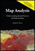
operations. For example, a Hugag is a
curious mythical beast (see figure 1) with strong preferences for terrain
configuration:
-
Prefers low elevations (severe nose bleeds at higher altitudes)
-
Prefers gentle slopes (fear of falling over and unable to get up)
-
Prefers southerly aspects (a place in the sun)
A
binary habitat model of Hugag preferences is the simplest to conceptualize and
implement. It is analogous to the manual
procedures for map analysis popularized in the book Design with Nature, by Ian L. McHarg,
first published in 1969. This seminal
work was the forbearer of modern map analysis by describing an overlay procedure
involving paper maps, transparent sheets and pens.
For
example, if avoiding steep slopes was an important decision criterion, a
draftsperson would tape a transparent sheet over a topographic map, delineate
areas of steep slopes (contour lines close together) and fill-in the
precipitous areas with an opaque color.
The process is repeated for other criteria, such as the Hugag’s preference to avoid areas that are
northerly-oriented and at high altitudes.
The annotated transparencies then are aligned on a light-table and the
“clear” areas showing through identify acceptable Hugag habitat.
Figure
1. The Hugag prefers low elevations, gentle
slopes and southerly aspects.
(see http://www.fearsomecreaturesofthelumberwoods.com/mainindex.htm
for more fearsome creatures)
An
analogous procedure can be implemented in a computer by using the value 0 to
represent the
unacceptable areas (opaque) and 1 to represent acceptable habit
(clear). As shown in figure 2, an Elevation map is used to derive a map of
terrain steepness (Slope_map)
and orientation (Aspect_map). A value of 0 is assigned to locations Hugags want to avoid—
Greater
than 1800 feet elevation = 0 …too high
Greater
than 30% slope = 0 …too steep
North,
northeast and northwest = 0 …to northerly
—with
all other locations assigned a value of 1 to indicate acceptable areas.
The
individual binary habit maps are shown in 3D and 2D displays on the right side
of figure 2. The dark red portions
identify unacceptable areas that are analogous to McHarg’s
opaque colored areas delineated on otherwise clear transparencies.
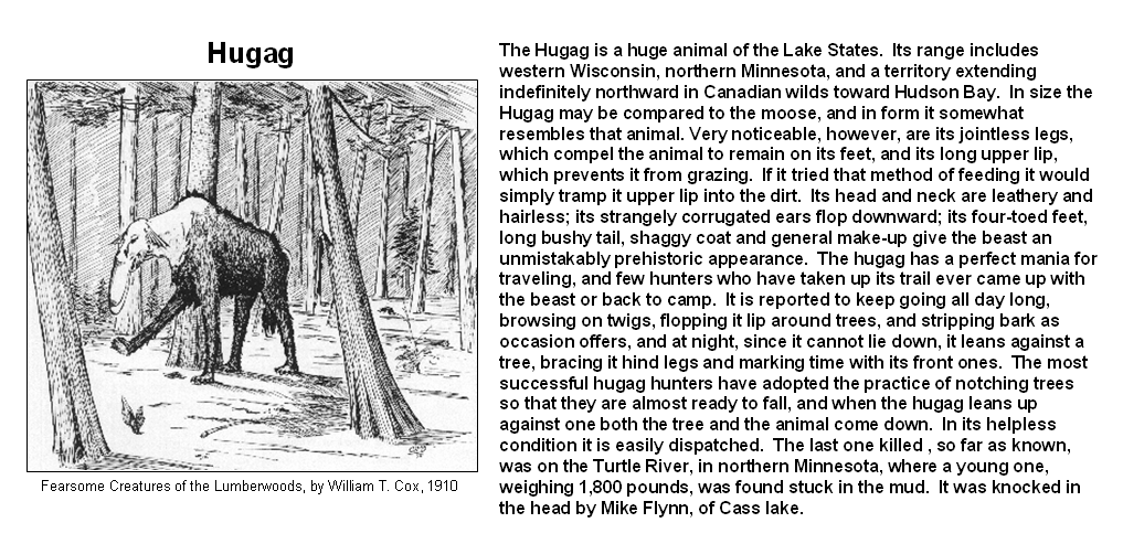
A Binary
Suitability map of Hugag habitat is generated by multiplying the three
individual binary preference maps (left side of figure 3). If a zero is encountered on any of the map
layers, the solution is sent to zero (bad habitat). For the example location on the right side of
the figure, the preference string of values is 1 * 1 * 0 = 0 (Bad). Only locations with 1 * 1 * 1 = 1 (Good)
identify areas without any limiting factors—good elevations, good slopes and
good orientation. These areas are
analogous to clear areas showing through the stack of transparencies.

Figure 2.
Binary maps representing Hugag preferences are coded as 1= good and 0=
bad.
While
this procedure mimics manual map processing, it is limited in the information
it generates. The solution is binary and
only differentiates acceptable and unacceptable locations. But isn’t an area that is totally bad (0 * 0
* 0 = 0) different from one that is just limited by one factor (1 * 1 * 0 =
0)? Two factors are acceptable thus
making it “nearly good.”
Figure
3. The binary habitat maps are multiplied
together to create a Binary Suitability map (good
or bad) or added together to create a
Ranking Suitability map (bad, marginal,
better or best).
The
right side of figure 3 shows a Ranking Suitability map of Hugag
habitat. In this instance the individual
binary maps are simply added together for a count of the number of acceptable
locations. Note that the areas of
perfectly acceptable habitat (light grey) on both the binary and ranking
suitability maps have the same geographic pattern. However, the unacceptable area on the ranking
suitability map contains values 0 through 2 indicating how many acceptable factors
occur at each location. The zero value
for the area in the northeastern portion of the map identifies very bad
conditions (0 + 0 + 0= 0). The example
location, on the other hand, is nearly good (1 + 1 + 0= 2).
Mapping
Techniques Rate Hugag Habitat Suitability
(GeoWorld, August 2004)
The
previous section described a couple of basic techniques for suitability
modeling— Binary and Ranking. Both procedures use “binary maps” that
identify just good (1) and bad (0) conditions on a set of criteria maps. In the example, three binary habitat maps
(good slopes, aspects and elevations) were multiplied together to create a Binary Suitability map (bad= any 0 or
good=1*1*1) or added together to create a Ranking
Suitability map (bad= 0+0+0= 0, marginal= 1, better= 2 or best= 1+1+1= 3).
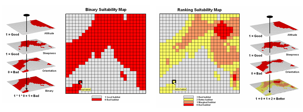
A
further extension of the binary techniques uses a mathematical trick. The criteria maps are reclassified to a
binary progression of numbers (1, 2 and 4) instead of all 1’s for acceptable
habitat (figure 1). When these maps are
summed the result is a unique value for each combination of values. For example, a location with a sum of 3 can
only occur if it is gently sloped (1) plus southerly exposed (2) plus too high
(0). The best habitat is indicated by
the value 7 (1+2+4= 7).
A Binary Progression Suitability map
contains a great deal of information beyond that of a simple binary or ranking
map as it indicates the actual combinations of acceptable and unacceptable
conditions. If there are more than three
criteria layers, the progression is just extended (…8, 16, 32, 64, etc.). In all cases the permutations result in a
unique sum.
However
all binary models suffer the same problem—things are either good or bad with no
degree of goodness. It’s like pass/not
pass grading that doesn’t distinguish exceptional performance (either good or
bad) and forces a sharp boundary instead of a gradient of performance.
Figure
1. Binary Progression Suitability map with
combinations indicated.
Figure
2 depicts an alternative procedure where each of criteria layers are “graded”
on a scale from 1= very bad to 9= very good.
For this example the calibration was—
Slope
Map: >40%=
1 (very bad); 30-40= 3; 20-30= 5; 10-20= 7; 0-10= 9 (very good)
Aspect Map: N, NE, NW= 1
(very bad); E, Flat= 5; W= 6; SE, S, SW= 9 (very good)
Elevation Map: >1800ft= 1 (very
bad); 1400-1800= 3; 1250-1400= 5; 900-1250= 7; 0-900= 9 (very good)
…then
the individual criteria maps are averaged for an overall score. In addition, lakes are masked as they
represent impossible habitat (drowned Hugags).
The
result is an Average Suitability map
containing an overall score for each map location. Note the results for the example location in
both figure 1 and 2. The Binary
Progression solution ranks it as totally acceptable (7= gentle, southerly,
low), while the Average Suitability solution rates it as mediocre habitat (5.3=
mid-range on a 1 to 9 scale). The dark
green locations, on the other hand, identify very good habitat (8-9 rating) and
the bright red locations indicate the worst habitat (1-2 rating).
Figure
2. Average Suitability map
with an average score for each location.
The continuous
gradient solution provides significantly more information than any of the
binary techniques. In practice, the
individual map layers are assigned weights to indicate their relative
importance and a weighted-average is computed.
The areas with high scores can be isolated and designated sensitive
habitat areas for natural resource planning.
Figure
3 shows the average suitability model applied to a larger area based on freely
available 30m digital elevation data.
When the suitability map is draped on the terrain surface its results
are easily evaluated. The best areas
(dark green) align with the gentle, southerly sloped and relatively low
areas. The worst areas (bright red)
align with steep northerly sloped and relatively high areas.
In
practical applications, habitat modeling considers many more factors than
simply terrain configuration. For
example, the model could be extended to evaluate the additional criterion that
“Hugags would prefer to be within or near forested
areas” (proximity to
Figure
3. Draping the Average Suitability map over the
Elevation surface shows good alignment with critical terrain features.
Keep in
mind that suitability modeling isn’t restricted to wildlife habitat
analysis. The approach is just as valid
for identifying “customer habitat” in geo-business, or crop suitability in
agriculture, or pipeline suitability for identifying the best route. Like statistics, the suitability modeling
cuts a wide swath through many applications as a fundamental analytical tool.
Logic and Extent Elevate Suitability Models to New Levels
(GeoWorld, October 2004)
The
previous sections on suitability modeling used wildlife habitat mapping to illustrate
the development of progressively more powerful modeling approaches—binary,
ranking, permutation and rating models.
All four approaches used the same set of basic criteria—Hugag preference
for gentle slopes, southerly aspects and lower elevations—as depicted in figure
1. The difference in how the processing
takes place was the focus of discussion.
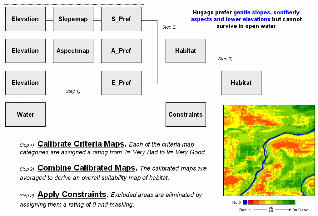
Figure
1. Model logic for basic Hugag
habitat suitability mapping.
In the
case of a binary model each
consideration is treated as either good or bad and results in a habitat map
that identifies just good and bad habitat areas. A ranking
model, on the other hand, uses the same good/bad criteria but identifies
the number of good factors for each map location with higher values indicating
increasingly higher habitat ranking. A permutation model provides even more
information by identifying the unique combination of good and bad factors
occurring at each location.
A rating model is the most powerful
approach. It breaks the good/bad
dichotomy into a gradient of preference most often expressed as 1= very bad to
9= very good. For example, the preference
for gentle slopes (S_Pref in figure 1) was assigned
as 1 (very bad) = >40%; 3= 30-40; 5= 20-30; 7= 10-20; and 9 (very good) =
0-10%. In a similar manner, categories
for aspect and elevation are calibrated then averaged and masked for constrained
areas to generate the overall suitability map shown in the figure. This result contains continuous habitat
values—considerably more information than simply the spatial coincidence of
discrete areas of good/bad classifications.
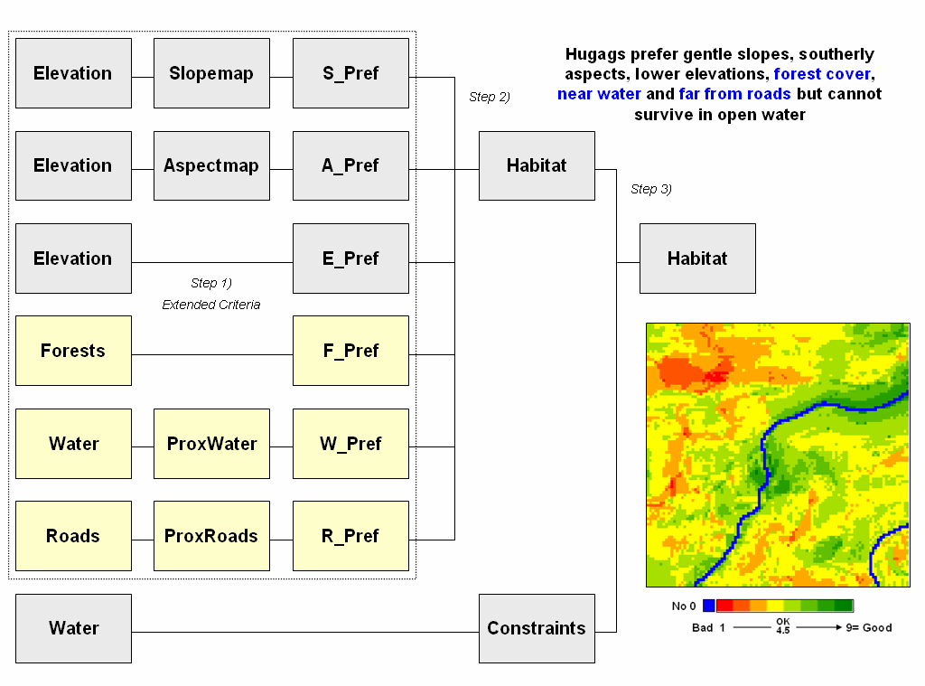
Figure
2. Extended model logic for
considering Hugag preference for being in forests, near water and far from
roads.
While
processing approach is an important consideration, the model logic and extent
can be even more important in determining model accuracy. In practical applications, the habitat model
would likely consider many more factors than simply terrain configuration. Figure 2 shows a flowchart of the extended
model logic to evaluate the additional criteria that “Hugags
would prefer to be in forested areas” (Forest map), that “Hugags
would prefer to be near water” (proximity to Water map) and that “Hugags would prefer to be far from roads” (proximity to
Roads map).
In
suitability modeling, these considerations are treated as separate sub-models
to derive the necessary criteria, then calibrated on the 1 to 9 preference
scale and averaged with the basic set of terrain considerations for an overall
habitat map shown in the figure.
Note
that a large part of the model’s strength or weakness is established in Step 1—calibrate criteria maps. As much as possible, the identification of
map criteria needs to reflect good science and/or expert opinion to capture
factors that are both important and easily measurable. Similarly, the calibration of the maps into
the 1-9 preference range needs to capture realistic relative values, not
whimsical or biased assignments.
Step2— combine calibrated maps is another area
requiring considerable understanding of the system being modeled. A simple average of the calibrated map layers
assumes that all of the criteria are equally important. The right inset in Figure 3 shows the habitat
results for expert thinking that Hugags are “10
times more concerned about slope, forest and water considerations than they are
about aspect, elevation and roads considerations.”
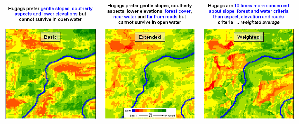
Figure
3. Habitat rating maps for progressively more
powerful model logic and processing.
The procedure for determining relative importance
involves computing the weighted-average of the six map layers. It is analogous to a professor’s grading some
exams more important than others in determining a class grade. In this case, the map values correspond to
student grades on each exam; each student is represented as a grid cell on the
map, kind of like their desk seats in the classroom floor plan.
Note the similarities and differences in the maps
induced by the additional criteria (Extended) and relative weighting of map
layers (Weighted). Provided expert
opinion is sound, the weighted map on the right would be considered the most
accurate representation of Hugag habitat.
Keep in mind that calibrating and weighting are
extremely critical steps in suitability modeling. Procedures, such as Delphi and AHP, can be
used to derive these factors in a quantitative, objective, consistent and
comprehensive manner (see Author’s Notes). In addition, purposeful changing these
factors can reflect different assumption scenarios analogous to “what if”
questions applied to traditional spreadsheet analysis.
From
this perspective, it is how the suitability maps change that becomes
information about the sensitivity of a project area to the interplay of
criteria, calibrations and weights.
This takes us well beyond mapping to assessing the spatial relationships
within a system and their logical expression within a GIS. As GIS technology matures, the focus is
shifting from simply access of static map products depicting physical features
for navigation and inventory to a dynamic environment that enables “thinking
with a stack maps” within decision-making contexts.
_____________________
(Back
to the Table of Contents)