|
Beyond
Mapping III Topic 3
– Basic Techniques in Spatial Analysis (Further Reading) |
Map Analysis book |
(Spatial Coincidence)
Key Concepts Characterize Unique
Conditions — describes a technique for handling unique combinations
of map layers (April 2006)
Use “Shadow Maps” to Understand
Overlay Errors — describes how shadow maps of certainty can be used
to estimate error and its propagation (September 2004)
<Click here> for a printer-friendly version of this topic (.pdf).
(Back
to the Table of Contents)
______________________________
Key
Concepts Characterize Unique Conditions
(GeoWorld, April
2006)
Back in the days of old
In these austere conditions programmers searched for algorithms and
data structures that saved nanoseconds and kilobytes. The concept of a Universal Polygon Coverage
was a mainstay in vector-based processing.
By smashing a stack of relatively static map layers together a single
map was generated that contained all of the son and daughter polygons. This “compute once/use many” approach had
significant efficiency gains as coincidence overlay was solved once then table
query and math simply summarized the combinations as needed.
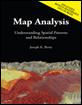
The top portion of figure 1 shows a simplified schematic of the
Universal Polygon approach. The lines
defining the individual polygons on the three vector maps are intersected
(analogous to throwing spaghetti on a wall) to identify various combinations of
the input conditions as depicted in the large map in the middle.
For example, consider the unique combination of A2, B1 and C1. The intersections of the lines identify nodes
that split the parent polygon boundaries into the segments defining the six son
and daughter polygons of the combined conditions. The result is a single spatial table
containing all of the original delineations plus the derived coincidence
overlay information. Its corresponding
attribute table can be easily searched for any combination of conditions and/or
mathematically manipulated to generate a new field in the table—fast and
efficient.
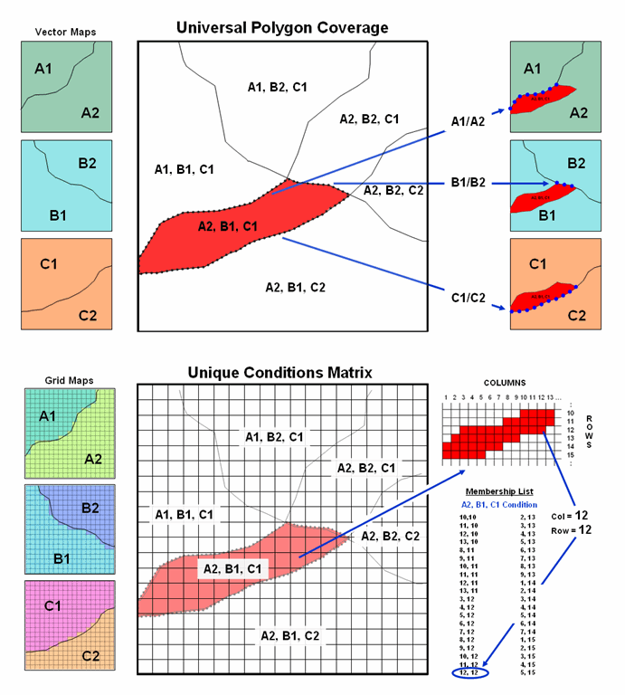
Figure 1. Comparison of the related concepts of
Universal Polygon Coverage (vector) and Unique Conditions Matrix (grid).
This pre-processing technique also works for grid-based data (bottom
portion of figure 1). The Unique
Conditions Matrix smashes a stack of grid layers together assigning a unique
value for each possible combination of conditions. For example, the A2, B1 and C1 combination
(termed a cohort) is defined by the grid cell block shown in the right portion
of the figure. Grid location column= 12
and row= 12 is one of the forty member cohort.
Figure 2 depicts a natural extension of the procedure involving two
tables—a Value Attribute Table and a Cohort Membership Table. For example, given grid layers for
travel-time for six stores classified into proximity classes (1= close, 2, 3
and 4= far) results in 4096 possible combinations. Each combination, in turn, forms a single
record (row) in the Value Attribute Table (VAT) file. The record contains a unique cohort ID number
and a field (column) for each of the base map conditions (figure 2, step
1). The user can operate on this table
to derive new information, such as the minimum travel-time to the closest
store, which is appended as a new field (step 2).
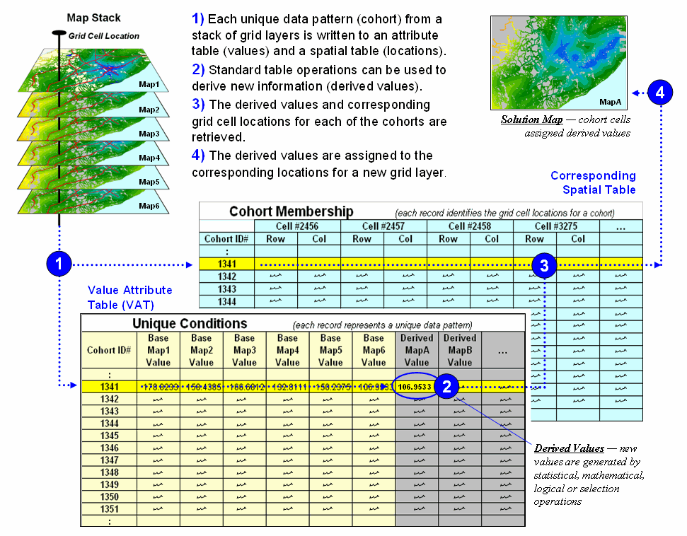
Figure 2. Steps linking unique conditions and cohort
membership tables for efficient and fast coincidence analysis.
Note that the VAT records identify unique conditions occurring anywhere
a project area whether the grid cells occur in few large clumps or widely
dispersed. The Cohort Membership Table
(CMT) contains a sting of values identifying the column/row coordinates for
each grid cell in the list. Thoughtful
organization of the list can implicitly carry information about the spatial
patterns within and among the cohorts of cells.
Step 3 links the attribute and spatial tables through their common ID
numbers. Any of the fields in the VAT
can be mapped by assigning the derived values to the cells defining each cohort
in the CMT (step 4).
Sounds easy and straight forward but there are a few caveats. First, the technique only addresses
point-by-point coincidence overlay and myopically ignores surrounding
conditions. Also, the conditions need to
be fairly stable, such as proximity and slope.
Finally, it requires continuous data to be reassigned into few discrete
classes on a relatively small number of map layers or the number of
combinations explodes. For example, 20
map layers with only four classification categories on each, results in over
sixteen million possible cohorts; a number that challenges most database
tables.
The advantage of the Unique Conditions technique in appropriate
application settings is that you calculate once (VAT) and use many
(CMT)—efficient and fast grid processing.
In the early years this was imperative for even the basic
Use “Shadow Maps” to Understand Overlay Errors
(GeoWorld,
September 2004)
Previous discussions in Topic 3 have focused on map overlay by
describing some of the procedures, considerations and applications. However, now is the moment of atonement—the
pitfalls of introduced error and its propagation. Keep in mind that there are two broad types
of errors in
Be realistic—soil or forest maps are just estimates of the actual
conditions and geographic patterns of these features. No one used a transit to survey the precise
and sharp boundary lines that delineate the implied distinct spatial objects. Soil and forest parcels aren’t discrete
things in either space or time and significant judgment is used in forcing
boundaries around them. Under some
conditions the guesses are pretty good; under other conditions, they can be
pretty bad. So how can the computer
“see” where things are good and bad?
That’s where the concept of a “shadow map of certainty” comes in and
directs attention to both the amount and pattern of map certainty. The left side of figure 1 depicts such an
information sandwich of a typical soil map with a shadow map of certainty glued
to its bottom. In this way the relative
certainty of the classification is known for each map location—look at the top
map to see the soil classification, then peer through to the bottom map to see
how likely that classification is at that location.
In this instance, any location with 100 meters of a soil boundary is
assigned only 50% certainty (orange) of correct classification while interior
areas of large features are assigned 100% certainty (grey). The assumption reflects the thought that
“there is a soil boundary around here somewhere, but I am just not sure exactly
where.”
A similar shadow map of certainty can be developed for the forest
information (right side of figure 1).
This simple estimate of certainty accounts for one photo interpreter
reaching out to add a tree along the edge of a parcel, and another interpreter
deciding not to. Both interpreters “see”
the interior of the forest parcel (certain) but discretion is used to form its
border (less certain). The 100m
certainty buffer reflects a bit of wiggle-room for interpretation.
Figure 1. Thematic maps with their corresponding shadow
maps of certainty. The orange areas indicate “less certain” areas (.50
probability) that are adjacent to a boundary.
Remote sensing classification, however, provides a great deal more
information about map certainty. For
example, the “maximum likelihood classifier” determines the probability that a
location is one of a number of different forest types using a library of
“spectral signatures” and multivariate statistics. In a sense the computer thinks “given the
color pattern for an area and knowledge of the various color patterns for
forest types in the area, which color most closely matches the appearance of
the area”—analogous to the manual interpretation process.
After a nanosecond or so, the computer decides which known pattern is
the closest, classifies it as that forest type, and then moves on to consider
the next grid cell. For example,
riparian and aspens tend to reflect lighter greens while pines and firs tend to
reflect darker greens. The import point is that the computer isn’t “seeing”
subtle color differences; it is analyzing numerical values to calculate the
probability that a location is one of any of the possible choices.
Traditionally, the approach simply chooses the most likely spectral signature,
classifies it, and then throws away the information on relative certainty of
the classification. Heck, the historical
objective was to produce a map, not data.
In addition, a spline function often is used to inscribe a seemingly
precise line around groups of similar classified cells so the results look more
like a manually drafted map. The result
is a set of spatially discrete objects implying perfect data for a warm and
fuzzy feeling, but disregarding the spatial resolution and classification probabilities
employed—sort of like throwing the bathwater out with the baby.
As
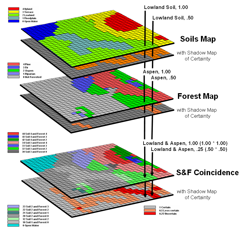
Figure 2. A shadow map of certainty for map overlay is
calculated by multiplying the individual certainty maps to derive a value
(joint probability) indicating the relative confidence in the coincidence among
map layers.
However, the real power of a shadow map of certainty is in addressing
processing errors that occur during map overlay. Common sense suggests that if you overlay a
fairly uncertain map with another fairly uncertain map, chances are the
resulting coincidence map is riddled with even more uncertainty. But the problem is more complex, as it is
dependent on the intersection of the unique spatial patterns of certainty of
the two (or more) maps.
Consider overlaying the soils and forest maps as depicted in figure
2. A simple map overlay considers just
the thematic map information and summarizes the coincidence between the two
maps. Note that both of the “speared”
locations identify Lowland soils occurring with
Now consider the effect of certainty propagation. The location on the left is certain on both
maps, so the coincidence is certain (1.00 *1.00= 1.00). However, the location on the right is less
certain on both maps, so the chance that it contains both lowland soils and
aspen is very uncertain certain (.50 * .50= .25).
The ability to quantify and account for map certainty is a critical
step in moving
____________________________
(Back to the Table of Contents)