|
Beyond
Mapping III Epilog
– The Many Faces of GIS (Further Reading) |
Map Analysis book |
(GIS Community Issues)
Is
GIS Technology Ahead of Science? — discusses several
issues surrounding the differences in the treatment of non-spatial and spatial
data (February
1999)
Observe
the Evolving GIS Mindset — illustrates the
"map-ematical" approach to analyzing mapped data (March 1999)
(GIS Education Considerations)
Where
Is GIS Education — describes the broadening appeal of
Varied
Applications Drive GIS Perspectives — discusses how
map analysis is enlarging the traditional view of mapping (August 1997)
Diverse
Student Needs Must Drive GIS Education — identifies
new demands and students that are molding the future of GIS education (September 1997)
Turning
GIS Education on Its Head — describes the numerous
GIS career pathways and the need to engage prospective students from a variety
of fields (May
2003)
<Click here> for a printer-friendly version of this topic (.pdf).
(Back
to the Table of Contents)
______________________________
Is
GIS Technology Ahead of Science?
(GeoWorld,
February 1999)
The movement from mapping to map analysis marks a turning point in the
collection and processing of geographic data.
It changes our perspective from “spatially-aggregated” descriptions and
images of an area to “site-specific” evaluation of the relationships among
mapped variables. The extension of the
basic map elements from points, lines and areas to map surfaces and the
quantitative treatment of these data has fueled the transition. However, this new perspective challenges the
conceptual differences between spatial and non-spatial data, their analysis and
scientific foundation.
For many it appears to propagate as many questions as it seems to answer. I recently had the opportunity to reflect on
the changes in spatial technology and its impact on science for a presentation*
before a group of scientists. Five
foundation-shaking questions emerged.
Is the “scientific method” relevant
in the data-rich age of knowledge engineering?
The first step in the scientific method is the statement of a
hypothesis. It reflects a “possible”
relationship or new understanding of a phenomenon. Once a hypothesis is established, a
methodology for testing it is developed.
The data needed for evaluation is collected and analyzed and, as a
result, the hypothesis is accepted or rejected.
Each completion of the process contributes to the body of science,
stimulates new hypotheses, and furthers knowledge.
The scientific method has served science well. Above all else, it is efficient in a
data-constrained environment. However,
technology has radically changed the nature of that environment. A spatial database is composed of thousands
upon thousands of spatially registered locations relating a diverse set of
variables.
In this data-rich environment, the focus of the scientific method shifts from
efficiency in data collection and analysis to the derivation of alternative
hypotheses. Hypothesis building results
from “mining” the data under various spatial, temporal and thematic
partitions. The radical change is that
the data collection and initial analysis steps precede the hypothesis
statement— in effect, turning the traditional scientific method on its head.
Is the “random thing” pertinent in
deriving mapped data
A cornerstone of traditional data analysis is randomness. In data collection it seeks to minimize the
effects of spatial autocorrelation and dependence among variables. Historically, a scientist could measure only
a few plots and randomness was needed to provide an unbiased sample for
estimating the typical state of a variable (i.e., average and
standard deviation).
For questions of central tendency, randomness is essential as it supports the
basic assumptions about analyzing data in numeric space, devoid of
“unexplained” spatial interactions.
However, in geographic space, randomness rarely exists and spatial
relationships are fundamental to site-specific management and research.
Adherence to the “random thing” runs counter to continuous spatial expression
of variables. This is particularly true
in sampling design. While efficiently
establishing the central tendency, random sampling often fails to consistently exam
the spatial pattern of variations. An
underlying systematic sampling design, such as systematic unaligned (see
Are geographic distributions a
natural extension of numerical distributions?
To characterize a variable in numeric space, density functions, such as
the standard normal curve, are used.
They translate the pattern of discrete measurements along a “number
line” into a continuous numeric distribution.
Statistics describing the functional form of the distribution determine
the central tendency of the variable and ultimately its probability of
occurrence. Consideration of additional
variables results in an N-dimensional numerical distribution visualized as a
series of scatterplots.
The geographic distribution of a variable can be derived from discrete sample
points positioned in geographic space.
Map generalization and spatial interpolation techniques can be used to
form a continuous distribution, in a manner analogous to deriving a numeric
distribution (see
Although the conceptual approaches are closely aligned, the information
contained in numeric and geographic distributions is different. Whereas numeric distributions provide insight
into the central tendency of a variable, geographic distributions provide
information about the geographic pattern of variations. Generally speaking, non-spatial
characterization supports a “spatially-aggregated” perspective, while spatial
characterization supports “site-specific” analysis. It can be argued that research using
non-spatial techniques provides minimal guidance for site-specific management—
in fact, it might be even dysfunctional.
Can spatial dependencies be modeled?
Non-spatial modeling, such as linear regressions derived from a set of
sample points, assumes spatially independent data and seeks to implement the
“best overall” action everywhere.
Site-specific management, on the other hand, assumes spatially dependent
data and seeks to evaluate “IF <spatial condition> THEN <spatial
action>” rules for the specific conditions throughout a management
area. Although the underlying
philosophies of the two approaches are at odds, the “mechanics” of their
expression spring from the same roots.
Within a traditional mathematical context, each map represents a “variable,”
each spatial unit represents a “case” and the value at that location represents
a “measurement.” In a sense, the map
locations can be conceptualized as a bunch of sample plots— it is just that
sample plots are everywhere (vis. cells in a gridded map surface). The result is a data structure that tracks
spatial autocorrelation and spatial dependency.
The structure can be conceptualized as a stack of maps with a vertical
pin spearing a sequence of values defining each variable for that location—
sort of a data shish kebab. Regression,
rule induction or a similar techniques, can be applied to the data to derive a
spatially dependent model of the relationship among the mapped variables.
Admittedly, imprecise, inaccurate or poorly modeled surfaces, can incorrectly
track the spatial relationships. But,
given good data, the “map-ematical” approach has the capability of
modeling the spatial character inherent in the data. What is needed is a concerted effort by the
scientific community to identify guidelines for spatial modeling and develop
techniques for assessing the accuracy of mapped data and the results of its
analysis.
How can “site-specific” analysis
contribute to the scientific body of knowledge?
Traditionally research has focused on intensive investigations
comprised of a limited number of samples.
These studies are well designed and executed by researchers who are
close to the data. As a result, the
science performed is both rigorous and professional. However, it is extremely tedious and limited
in both time and space. The findings
might accurately reflect relationships for the experimental plots during the
study period, but offer minimal information for a land manager 70 miles away
under different conditions, such as biological agents, soil, terrain and
climate.
Land managers, on the other hand, supervise large tracks of land for long
periods of time, but are generally unaccustomed to administering scientific
projects. As a result, general
operations and scientific studies have been viewed as different beasts. Scientists and managers each do their own
thing and a somewhat nebulous step of “technology transfer” hopefully links the
two.
Within today’s data-rich environment, things appear to be changing. Managers now have access to databases and
analysis capabilities far beyond those of scientists just a few years ago. Also, their data extends over a spectrum of
conditions that can’t be matched by traditional experimental plots. But often overlooked is the reality that
these operational data sets form the scientific fodder needed to build the
spatial relationships demanded by site-specific management.
Spatial technology has changed forever land management operations— now it is
destined to change research. A close
alliance between researchers and managers is the key. Without it, constrained research (viz.
esoteric) mismatches the needs of evolving technology, and heuristic (viz.
unscientific) rules-of-thumb are substituted.
Although mapping and “free association” geo-query clearly stimulates
thinking, it rarely contains the rigor needed to materially advance scientific
knowledge. Under these conditions a
data-rich environment can be an information-poor substitute for good science.
So where do we go from here?
In the new world of spatial technology the land manager has the
comprehensive database and the researcher has the methodology for its analysis—
both are key factors in successfully unlocking the relationships needed for
site-specific management. In a sense,
technology is ahead of science, sort of the cart before the horse. A
______________________
 Author’s
Note: This
column is based on a keynote address for the Site-Specific Management of Wheat
Conference, Denver, Colorado, March 4-5, 1998; a copy of the full text is
online at www.innovativegis.com/basis,
select Presentations & Papers.
Author’s
Note: This
column is based on a keynote address for the Site-Specific Management of Wheat
Conference, Denver, Colorado, March 4-5, 1998; a copy of the full text is
online at www.innovativegis.com/basis,
select Presentations & Papers.
Observe the Evolving GIS Mindset
(GeoWorld, July
2011)
A couple of seemingly ordinary events got me thinking about the
evolution of
I recently attended an open house for a local
The expanded community has brought a refreshing sense of practicality and
realism. The days of “
That brings up the other event that got me thinking. It was an email that posed an interesting
question…
“We are
trying to solve a problem in land use design using a raster-based
The problem involves “map-ematical reasoning” since there isn’t
a button called “identify the most suitable land use” in any of the
Figure 1. Schematic of the problem to identify the most
suitable land use for each location from a set of grid layers.
That’s simple for you, but computers and
Step 1. Find the maximum value at each grid location on the set of
input maps—
COMPUTE Residential_Map maximum Golf_Map
maximum Conservation_Map for Max_Value_Map
Step 2. Compute the difference between an input map and the
Max_Value_Map—
COMPUTE Residential_Map minus Max_Value_Map for Residential_Difference_Map
Step 3. Reclassify the difference map to isolate locations where
the input map value is equal to the maximum value of the map set (renumber maps
using a binary progression; 1, 2, 4, 8, 16, etc.)—
RENUMBER Residential_Difference_Map for Residential_Max1_Map
assigning 0 to -10000 thru -1 (any negative number; residential
less than max_value)
assigning 1 to 0 (residential
value equals max_value)
Step 4. Repeat steps 2-3 for the other input maps—
… Golf_Max2_Map using 2 and Conservation_Max4_Map using 4 to
identify areas of maximum suitability for each grid layer
Step 5. Combine individual "maximum" maps and label the
“solution” map—
COMPUTE Residential_Max1_Map plus Golf_max2_Map plus Conservation_Max4_Map
for Suitable_Landuse_Map
LABLE Suitable_Landuse_Map
1 Residential (1
+ 0 + 0)
2 Golf Course (0
+ 2 + 0)
4 Conservation (0
+ 0 + 4)
3 Residential and Golf Course Tie (1
+ 2 + 0)
5 Residential and Conservation Tie (1 + 0 +
4)
6 Golf Course and Conservation Tie (0 + 2 + 4)
7 Residential, Golf Course and
Conservation Tie (1 + 2 +
4)
Note: the sum of a binary
progression of numbers assigns a unique value to all possible combinations.
OK, how many of you map-ematically reasoned the above solution, or
something like it? Or thought of
extensions, like a procedure that would identify exactly “how suitable” the
most suitable land use is (info is locked in the Max_Value_Map; 76 for the
top-left cell and 87 for the bottom right cell). Or generating a map that indicates how much
more suitable the maximum land use is for each cell (the info is locked in the
individual Difference_Maps; 56-76= -20 for Golf as the runner up in the
top-left cell). Or thought of how you
might derive a map that indicates how variable the land use suitabilities are
for each location (info is locked in the input maps; calculate the coefficient
of variation [[stdev/mean]*100] for each grid cell).
This brings me back to the original discussion.
It’s true that the rapid growth of
However, in many instances the focus has shifted from the analysis-centric
perspective of the original “insiders” to a data-centric one shared by a
diverse set of users. As a result, the
bulk of current applications involve spatially-aggregated thematic mapping and
geo-query verses the site-specific models of the previous era. This is good, as finally, the stage is set
for a quantum leap in the application of
Where Is GIS Education
(GeoWorld, June
1997)
When coupled with a cell phone, they can call for help and their
rescuers will triangulate on the signal and deliver a gallon of gas and an
extra large pizza within the hour. Whether you are a lost explorer near the
edge of the earth or soul-searching on your Harley, finding yourself has never
been easier—the revolution of the digital map is firmly in place.
A new-age real estate agent can search the local multiple listing for suitable
houses, then electronically “post” them to a map of the city. A few more mouse-clicks allows a prospective
buyer to take a video tour of the homes and, through a
However, the “intellectual glue” supporting such Orwellian mapping and
management applications of
The classical administrator’s response is to stifle the profusion of autonomous
Keep in mind the old adage that “the fighting at universities is so
fierce, because the stakes are so small.”
Acquisition of space and equipment are viewed less as a communal good,
as they are viewed as one department’s evil triumph over the others. My nine years as an associate dean hasn’t
embittered me, as much as it has ingrained organizational realities. Bruises and scar tissue suggest that the
efficiencies and cost savings of a centralized approach to
As with other aspects of campus life,
Assuming a balance can be met between efficiency and effectiveness of its
logistical trappings, the issue of what
The result is a patchwork of
The underlying theory and broader scope of the technology, however, can be lost
in the practical translation. While
geodetic datum and map projections might dominate one course (map-centric),
sequential query language and operating system procedures may dominate another
(data-centric). A third, application-oriented course likely skims both
theoretical bases (the sponge cake framework), then quickly moves to its
directed applications (the icing).
While academicians argue their relative positions in seeking the
“universal truth in
Varied
Applications Drive GIS Perspectives
(GeoWorld, August
1997)
Our struggles in defining
We have been mapping and managing spatial data for a long time. The earliest systems involved file cabinets
of information which were linked to maps on the wall through shoe leather. An early “database-entry, geo-search” of
these data required a user to sort through the folders, identify the ones of
interest, then locate their corresponding features on the map on the wall. If a map of the parcels were needed, a clear
transparency and tracing skills were called into play.
A “map-entry, geo-search” reversed the process, requiring the user to
identify the parcels of interest on the map, then walk to the cabinets to
locate the corresponding folders and type-up a summary report. The mapping and data management capabilities
of
This new perspective of spatial data is destined to change our paradigm of map
analysis, as much as it changes our procedures.
As depicted in figure 1,
Figure 1. Various approaches used in
The numerical treatment of maps, in turn, takes two basic forms—spatial
statistics and spatial analysis. Broadly
defined, spatial statistics involves statistical relationships
characterizing geographic space in both descriptive and predictive terms. A familiar example is spatial interpolation
of point data into map surfaces, such as weather station readings into maps of
temperature and barometric pressure.
Less familiar applications might use data clustering techniques to
delineate areas of similar vegetative cover, soil conditions and terrain
configuration characteristics for ecological modeling. Or, in a similar fashion, clusters of
comparable demographics, housing prices and proximity to roads might be used in
retail siting models.
Spatial analysis, on the other hand, involves characterizing
spatial relationships based on relative positioning within geographic space. Buffering and topological overlay are
familiar examples. Effective distance,
optimal path(s), visual connectivity and landscape variability analyses are
less familiar examples. As with spatial
statistics, spatial analysis can be based on relationships within a single map
(univariate), or among sets of maps (multivariate). As with all new disciplines, the various
types of
In all cases,
Diverse Student Needs Must Drive GIS Education
(GeoWorld,
September 1997)
Fundamental to understanding
Several concepts, however, represent radical shifts in the spatial
paradigm. Take the concept of map
scale. It’s a cornerstone to traditional
mapping, but it doesn’t even exist in a
Similarly, combining maps with different data types, such as multiplying the
ordinal numbers on one map times the interval numbers on another, is
map-ematical suicide. Or evaluating a
linear regression model using mapped variables expressed as logarithmic values,
such as a PH for soil acidity. Or
consider overlaying five fairly accurate maps (good data in) whose uncertainty
and error propagation results in large areas of erroneous combinations (garbage
out). It is imperative that
The practicalities of implementing procedures often overshadow their
realities. For instance, it’s easy to
use a ruler to measure distances, but its measurements are practically useless.
The assumption that everything moves in a straight line does not square with
real-world—“as the crow flies,” in reality, rarely follows a straightedge. Within a
In practice, a 100 foot buffer around all streams is simple to establish (as
well as conceptualize), but has minimal bearing on actual sediment and
pollutant transport. It’s common sense
that locations along a stream that are steep, bare and highly erodeable should
have a larger setback. A variable-width buffer respecting intervening
conditions is more realistic.
Similarly, landscape fragmentation has been ignored in resource
management. It’s not that fragmentation
is unimportant, but too difficult to assess until new
These new procedures and the paradigm shift are challenging
The diversity of users, however, often is ignored in a quest for a
“standard, core curriculum.” In so
doing, a casual user interested in geo-business applications is overwhelmed
with data-centric minutia; while the database manager receives to little. Although a standard curriculum insures common
exposure, it’s like forcing a caramel-chewy enthusiast to eat a whole box of
assorted chocolates. The didactic,
two-step educational approach (intro then next) is out-of-step with today’s
over-crowded schedules and the diversity
A potential user’s situation has a bearing on
Although non-traditional students tend to be older and even less patient, they
have a lot in common with the current wave of “out-of-step” traditional
students. They have even less time and
interest in semester-long “intro/next” course sequences. By default, vocational
training sessions are substituted for their
A mixed audience of traditional and non-traditional students provides
an engaging mixture of experiences. So
what’s wrong with this picture? What’s missing?
Not money as you might guess, but an end run around institutional
inertia and rigid barriers. Adoption of
________________________________
Author’s Note: the first three sections of this series on
Turning GIS Education on Its Head
(GeoWorld, May
2003)
Now that
As much as its technological underpinnings have changed,
In the 1990s several factors converged—sort of a perfect storm for
The early environments kept
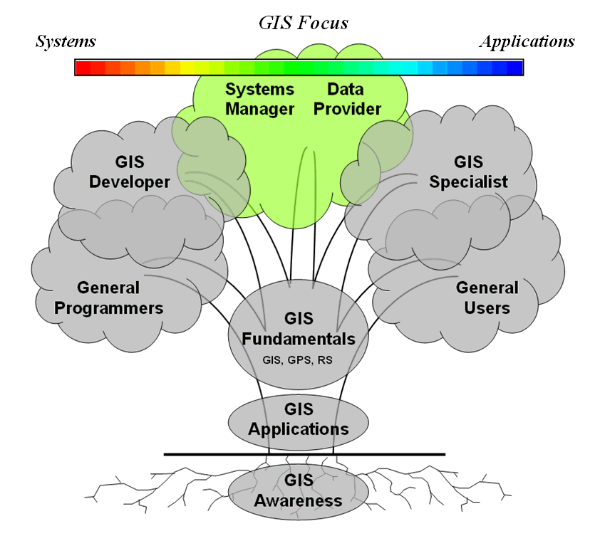
Figure 1. The
Figure 1 characterizes the
For example, the perspectives, skill sets and
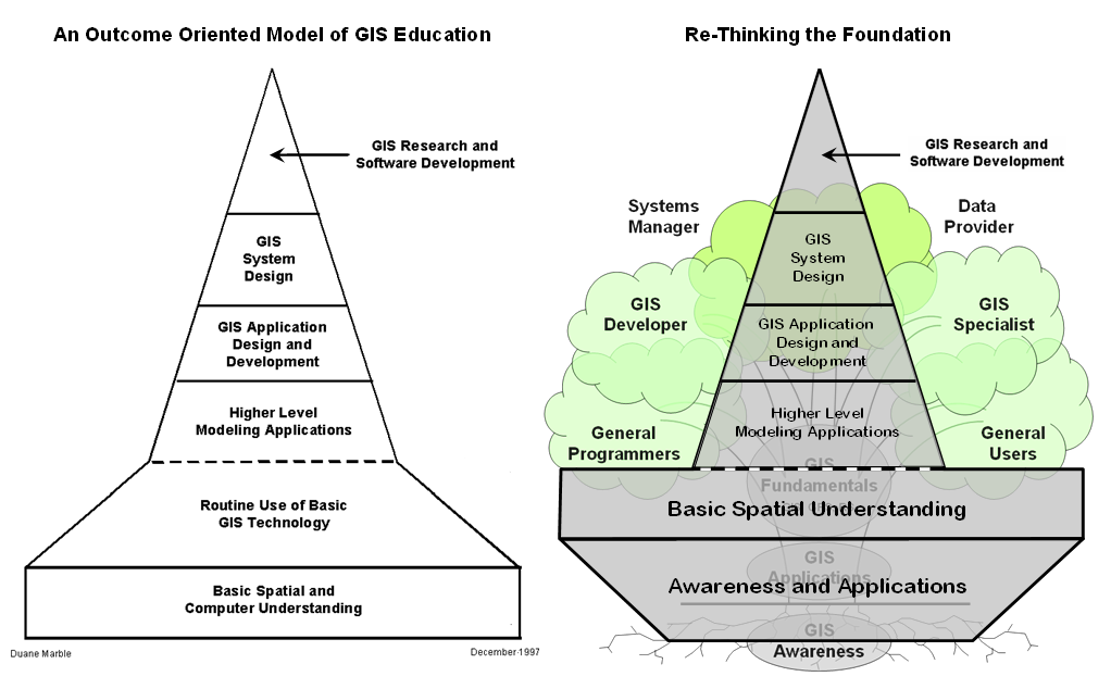
Figure 2.
Professor Marble with
These points are very well taken and reflect the evolution of most disciplines
crossing the chasm from start-up science to a popular technology. Marble suggests the solution “…appears to be
to devise a rigorous yet useful first course that will provide a sound initial
foundation for individuals who want to learn
So how can
The right-side of figure 2 turns the early phases of
Such experience wouldn't be a rice-cake flurry of "dog-and-pony show"
applications (e.g., frog habitat modeling in
That means that the next piece of the
The "up-side-down" approach suggests that the growing pool of
potential new users are first introduced to what
_________________
Author's Note: See Marble,
Duane F. 1997. Rebuilding the Top of the Pyramid: Structuring
http://www.ncgia.ucsb.edu/conf/gishe97/program_files/papers/marble/marble.html.
Author’s Update: (9/09) Duane Marble in a more recent thoughtful
article entitled “Defining the Components of the Geospatial Workforce—Who Are
We?” published in ArcNews, Winter 2005/2006, suggests that—
“Presently,
far too many academic programs concentrate on imparting only basic skills in
the manipulation of existing GIS software to the near exclusion of problem
identification and solving; mastery of analytic geospatial tools; and critical
topics in the fields of computer science, mathematics and statistics, and information
technology.”
http://www.esri.com/news/arcnews/winter0506articles/defining1of2.html
This
dichotomy of “tools” versus “science” is reminisce of the “-ists and -ologists”
debates involving differing perspectives of geotechnology in the 1990’s. For a discussion of this issue see Beyond
Mapping III, Epilog, “Melding the Minds of the “-ists” and “-ologists.”
available at:
http://www.innovativegis.com/basis/MapAnalysis/MA_Epilog/MA_Epilog.htm#Melding_Minds.
Other
related postings are at:
-
http://www.innovativegis.com/basis/present/GIS_Rockies09/GISTR09_Panel.pdf,
handout for the panel on “GIS Career Opportunities,” GIS in
the Rockies, Loveland, Colorado; September 16-18, 2009.
-
http://www.innovativegis.com/basis/present/LocationIntelligence09/LocationIntelligence09.pdf
, handout for the panel on
“Geospatial Jobs and the 2009 Economy,” Location Intelligence
Conference, Denver, Colorado, October 5-7, 2009.
-
http://www.innovativegis.com/basis/present/imagine97/,
a keynote address on “Education, Vocation and Enlightenment,” IMAGINE
Forum, Lansing, Michigan, May 1997.
(Back to the Table of Contents)