Beyond Mapping
|
Map
Analysis book with companion CD-ROM for hands-on exercises and further reading |
Lumpers and Splitters Propel GIS
— describes the
two camps of GIS (GeoExploration and GeoScience)
The Softer Side of GIS
— describes a
Manual GIS (circa 1950) and the relationship between social science conceptual
frameworks for understanding/judgment in GIS modeling
Melding the Minds of the “-ists”
and “-ologists”
— elaborates on
the two basic mindsets driving the geotechnology community
Is GIS Technology Ahead of Science?
— discusses
several issues surrounding the differences in the treatment of non-spatial and
spatial data
The Good, the Bad and the Ugly
Sides of GIS — discusses
the potential of geotechnology to hinder (or even thwart) societal progress
Where Do We Go from Here?
— Swan Song
after 25 years of Beyond Mapping columns
Note: The processing and figures discussed in this topic were derived using MapCalcTM
software. See www.innovativegis.com to download a
free MapCalc Learner version with tutorial materials for classroom and
self-learning map analysis concepts and procedures.
<Click here> right-click to download a
printer-friendly version of this topic (.pdf).
(Back to
the Table of Contents)
______________________________
Lumpers and Splitters Propel
(GeoWorld, December, 2007)
Earlier discussions have focused on the numerical nature of GIS data (GeoWorld Sep-Nov, 2007; Topic 7 in the online Beyond Mapping III compilation at http://www.innovativegis.com/basis/MapAnalysis). The discussions challenged the traditional assumption that all data are “normally” distributed suggesting that most spatial data are skewed and that the Median and Quartile Range often are better descriptive statistics than the Mean and Standard Deviation.
Such heresy was followed by an assertion that any central tendency statistic tends to overly generalize and often conceal inherent spatial patterns and relationships within nearly all field collected data. In most applications, Surface Modeling techniques, such as density analysis and spatial interpolation, can be applied to derive the spatial distribution of a set of point-sampled data.
Figure 1 outlines the major points of the earlier discussion. The left side of the figure depicts Desktop Mapping’s approach that reduces a set of field data to a single representative value that is assumed to be everywhere the same within each polygon (Discrete Spatial Object). Each parcel is “painted” with an appropriate color indicating the typical value—with darker green indicating a slightly lower average value derived from numerous samples falling within the polygon.
Map Analysis’s approach, on the other hand, establishes a spatial gradient based on the relative positions and values of the point-sampled data (Continuous Spatial Distribution). A color ramp is used to display the continuum of estimated values throughout each parcel—light green (low) to red (high). Note that the continuous representation identifies a cluster of extremely high values in the upper center portion of the combined parcels that is concealed by the discrete thematic mapping of the averages.
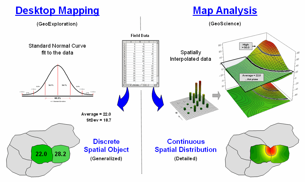
Figure 1. A data set can be characterized
both discretely and continuously to derive different perspectives of spatial
patterns and relationships.
OK, so much for review …what about the big picture? The discussion points to today’s convergent trajectory of two GIS camps— GeoExploration and GeoScience. Traditional computer companies like Google, Microsoft and Yahoo are entering the waters of geotechnology at the GeoExploration shallow end. Conversely, GIS vendors with deep keels in GeoScience are capitalizing on computer science advances for improved performance, interoperability and visualization.
An important lesson learned by the GeoScience camp is that data has to be integrated with a solution and not left as an afterthought for users to cobble together. Another lesson has been that user interfaces need to be intuitive, uncluttered and consistent across the industry. Additionally, the abstract 2D pastel map is giving way to 3D visualization and virtual reality renderings— a bit of influence from our CAD cousins and the video game industry.
But what are the take-aways for traditional computer science vendors? First and foremost is an active awareness of the breadth of geotechnology, both in terms of its technical requirements and its business potential. Under the current yardstick of “eyeball contacts,” GeoExploration tools have been wildly successful.
But at the core, have recent technological advancements really changed mapping? …or has the wave of GeoExploration tools just changed mapping’s expression and access? …has the GIS evolution topped (or bottomed) out? …what about the future?
Current revolutionary steps in analytics and concepts are underway like the energized paddling beneath a seemingly serene swan. As a broad-brush framework for discussion of where we are heading, recall from your academic days the Philosopher’s Progression of Understanding shown in figure 2. It suggests that are differences between the spatial Data/Information describing geographic phenomena and the Knowledge/Wisdom needed for prescribing management action that solve complex spatial problems.
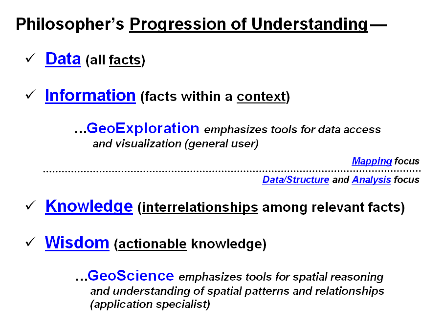
Figure 2. The two broad camps of
geotechnology occupy different portions of the philosopher’s progression of
understanding.
Most GeoExploration applications simply assemble spatial data into graphic form. While it might be a knock-your-socks-off graphic, the distillation of the data to information is left to visceral viewing and human interpretation and judgment (emphasizing Data and Information).
For example, a mash-up of a set of virtual pins representing crimes in a city can be poked into a Google Earth display. Interpretation and assessment of the general pattern, however, is left for the brain to construe. But there is a multitude of analytics that can be brought into play that translates the spatial data into information, knowledge and wisdom needed for decision-making. Geo-query can segment by the type of crime; density analysis can isolate unusually high and low pockets of crime; coincident statistics can search for correlation with other data layers; effective distance can determine proximity to key features; spatial data mining can derive prediction models.
While the leap from mapping to map analysis might be well known to those in GeoScience, it represents a bold new frontier to the GeoExploration camp. It suggests future development of solutions that stimulate spatial reasoning through “thinking with maps” (Information and Knowledge) rather than just visualizing data— a significant movement beyond mapping.
In part, the differences between the GeoExploration
and GeoScience camps parallel society’s age-old
dichotomy of problem perception—lumpers and
splitters. A "lumper"
takes a broad view assuming that details of a problem are not as important as
overall trends ...a picture is worth a thousand words (holistic). A "splitter" takes a detailed view
of the interplay among problem elements ...a model links thousands of pieces
(atomistic).
So how does all
this playout in geotechnology’s future? The two camps are symbiotic and can’t survive
without each other; sort of like Ralph and Alice Kramden
in The Honeymooners. GeoExploration
fuels the fire of mass acceptance, and in large part finances technology
development through billions of mapping clicks (General User; access and
visualization). GeoScience
lubricantes the wheels of advancement by developing
new data structures, analytical tools and applications (Application Specialist;
spatial reasoning and understanding).
It’s important to
note that neither camp is stationary and that they are continually evolving as
we move beyond traditional mapping. A
large portion of the mystique and influence of application specialists just a
few years ago are now commonplace on the desks (and handheld devices) of the
general public. Similarly, the flat,
pastel colored maps of just a few years ago have given away to interactive 3D
displays. While there will always be the
lumpers and splitters differences in perspective,
their contributions to the stone soup of geotechnology are equally
valuable—actually invaluable.
The Softer Side of GIS
(GeoWorld, January, 2008)
While computer-based procedures supporting Desktop Mapping seem revolutionary, the idea of linking descriptive information (What) with maps (Where) has been around for quite awhile. For example, consider the manual GIS that my father used in the 1950s outlined in figure 1.
The heart of the system was a specially designed index card that had a series of numbered holes around its edge with a comment area in the middle. In a way it was like a 3x5 inch recipe card, just a little larger and more room for entering information. For my father, a consulting forester, that meant recording timber stand information, such as area, dominant tree type, height, density, soil type and the like, for the forest parcels he examined in the field (What). Aerial photos were used to delineate the forest parcels on a corresponding map tacked to a nearby wall (Where).
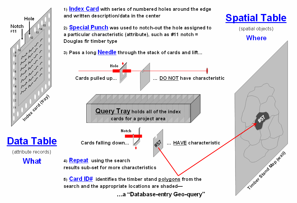
Figure
1. Outline of the processing flow of a manual GIS, circa 1950.
What went on between
the index card and the map was revolutionary for the time. The information in the center was coded and
transferred to the edge by punching out (notching) the appropriate numbered
holes. For example, hole
#11 would be notched to identify a Douglas fir timber stand. Another card would be notched at hole #12 to indicate a different parcel containing ponderosa
pine. The trick was to establish a
mutually exclusive classification scheme that corresponded to the numbered
holes for all of the possible inventory descriptors and then notch each card to
reflect the information for a particular parcel.
Cards for hundreds
of timber stands were indiscriminately placed in a tray. Passing a long needle through an appropriate
hole and then lifting and shaking the stack caused all of the parcels with a
particular characteristic to fallout— an analogous result to a simple SQL query
to a digital database. Realigning the
subset of cards and passing the needle through another hole then shaking would
execute a sequenced query—such as Douglas fir (#11) AND Cohasset soil
(#28).
The resultant card
set identified the parcels satisfying a specific query (What). The parcel ID# on each card corresponded to a
map parcel on the wall. A thin paper
sheet was placed over the base map and the boundaries for the parcels traced
and color-filled (Where)—a “database-entry geo-query.” A “map-entry geo-query,” such as identifying
all parcels abutting a stream was achieved by viewing the map, is achieved by
noting the parcel ID#’s on the map and searching with the needle to subset the
abutting parcels to get their characteristics.
The old days wore
out a lot of shoe leather running between the index card tray and the map
tacked to the wall. Today, it’s just electrons scurrying about in a computer at
gigahertz speed. However, the bottom
line is that the geo-query/mapping approach hasn’t changed
substantially—linking “What is Where” for a set of pre-defined parcels and
their stored descriptors. But the future
of GIS holds entirely new spatial analysis capabilities way outside our paper
map legacy.
Figure
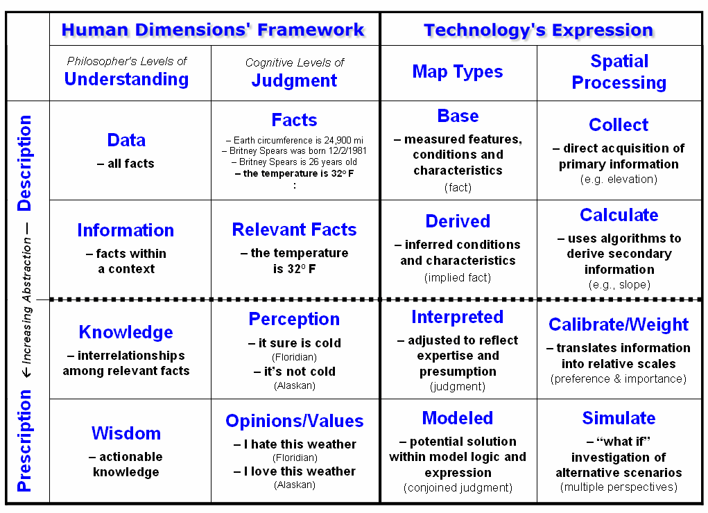
2. Conceptual framework for moving maps from Description to Prescription
application.
Figure 2 graphically
relates the softer (human dimensions) and harder (technology) sides of
GIS. The matrix is the result of musing
over some things lodged in my psyche years ago when I was a grad student (see
Author’s Note 1). Last month’s column
(December 2007) described the Philosopher’s Levels of Understanding
(first column) that moves thinking from descriptive Data, to relevant Information,
to Knowledge of interrelationships
and finally to prescriptive Wisdom
that forms the basis for effective decision-making. The dotted horizontal line in the progression
identifies the leap from visualization and visceral interpretation in GeoExploration of Data and Information to the map analysis
ingrained in GeoScience for gaining Knowledge and Wisdom
for problem solving.
The second column extends the gradient of Understanding to the stark reality of Judgment that complicates most decision-making applications of GIS. The basic descriptive level for Facts is analogous to that of Data and includes things that we know, such as the circumference of the earth, Brittney Spears’ birth date, her age and today’s temperature. Relevant Facts correspond to Information encompassing only those facts that pertain to a particular concern, such as today’s temperature of 32oF.
It is at the next two levels that the Understanding and Judgment frameworks diverge and translate into radically different GIS modeling environments. Knowledge implies certainty of relationships and forms the basis of science—discovery of scientific truths. The concept of Perception, however, is a bit mushier as it involves beliefs and preferences based on experience, socialization and culture—development of perspective. For example, a Floridian might feel that 32o is really cold, while an Alaskan feels it certainly is not cold, in fact rather mild. Neither of the interpretations is wrong and both diametrically opposing perceptions are valid.
The highest level of Opinion/Values implies actionable beliefs that reflect preferences, not universal truths. For example, the Floridian might hate the 32o weather, whereas the Alaskan loves it. This stark dichotomy of beliefs presents a real problem for many GIS technologists as the bulk of their education and experience was on the techy side of campus, where mapping is defined as precise placement of physical features (description of facts). But the other side of campus is used to dealing with opposing “truths” in judgment and sees maps as more fluid, cognitive drawings (prescription of relationships).
The columns on the right attempt to relate the dimensions of Understanding and Judgment to Map Types and Spatial Processing used in prescriptive mapping. The descriptive levels are well known to GIS’ers—Base maps from field collected data (e.g., elevation) and Derived maps calculated by analytical tools (e.g., slope from elevation).
Interpreted maps, on the other hand, calibrate Base/Derived map layers in terms of their perceived impact on a spatial solution. For example, gentle slopes might be preferred for powerline routing (assigned a value of 1) with increasing steepness less preferred (assign values 2 through 9) and very steep slopes prohibitive (assign 0). A similar preference scale might be calibrated for a preference to avoid locations of high Visual Exposure, in or near Sensitive Areas, far from Roads or having high Housing Density. In turn, the model criteria are weighted in terms of their relative importance to the overall solution, such as a homeowner’s perception that Housing Density and Visual Exposure preference ratings are ten times more important than Sensitive Areas and Road Proximity ratings (see Author’s Note 2).
Interpreted maps provide a foothold for tracking divergent assumptions and interpretations surrounding a spatially dependent decision. Modeled maps put it all together by simulating an array of opinions and values held by different stakeholder groups involved with a particular issue, such as homeowners, power companies and environmentalists concerns about routing a new powerline.
The Understanding progression assumes common truths/agreement at each step (more a natural science paradigm), whereas the Judgment progression allows differences in opinion/beliefs (more a social science paradigm). GIS modeling needs to recognize and embrace both perspectives for effective spatial solutions tuned to different applications. From the softer side perspective, GIS isn’t so much a map, as it is the change in a series of maps reflecting valid but differing sets of perceptions, opinions and values. Where these maps agree and disagree becomes the fodder for enlightened discussion, and eventually an effective decision. Judgment-based GIS modeling tends to fly in the face of traditional mapping— maps that change with opinion sound outrageous and are radically different from our paper map legacy and the manual GIS of old. It suggests a fundamental change in our paradigm of maps, their use and conjoined impact—are you ready?
_____________________________
Author’s Notes: 1) Ross Whaley, Professor Emeritus at
SUNY-Syracuse and member of my doctoral committee, in a plenary presentation at
the New York State
Melding the Minds of the “-ists” and “-ologists”
(GeoWorld, July 2009)
I recently attended the GIS in Higher Education Summit for Colorado Universities that wrestled with challenges and opportunities facing academic programs in light of the rapid growth of the geographic information industry and its plethora of commercial and government agency expressions. Geotechnology’s “mega-technology status” alongside the giants of Nanotechnology and Biotechnology seems to be both a blessing and a curse. The Summit’s take-away for me was that, while the field is poised for exponential growth, our current narrow footing is a bit unstable for such a giant leap.
Duane Marble in a thoughtful article (Defining the Components of the Geospatial Workforce—Who Are We?; ArcNews, Winter 2005/2006) suggests that—
“Presently,
far too many academic programs concentrate on imparting only basic skills in
the manipulation of existing GIS software to the near exclusion of problem
identification and solving; mastery of analytic geospatial tools; and critical
topics in the fields of computer science, mathematics and statistics, and
information technology.”
This dichotomy of “tools” versus
“science” is reminisce of the “-ists and -ologists” Wars of the 1990’s. While not on the same level as the Peloponnesian War that reshaped Ancient Greece, the two conflicts
have some parallels. The pragmatic and
dogged Spartans (an oligarchy) soundly trounced the intellectual and aristocratic
Athenians (a democracy). However in the
process, the economic toll was staggering, poverty widespread, cultures devastated and civil war
became a common occurrence throughout the Greek world that never recovered its
grandeur.
Figure 1. A civilized and gracious tension exists
between the of-the-tool and of-the-application groups.
Figure 1 portrays a similar, yet more civilized and gracious tension noted
during the Education Summit. The “-ists” in the
group pragmatically focused on programs emphasizing a GIS specialist’s command
of the tools needed to display, query and process spatial data (Data and
Information focus). The “-ologists,” on
the other hand, had a broader vision of engaging users (e.g., ecologists,
sociologists, hydrologists, epidemiologists, etc.) who understand the science
behind the spatial relationships that support decision-making (Knowledge and
Wisdom focus).
My first encounter with the “-ists” and “-ologists” conflict involved the U.S. Forest Service’s Project 615 in the early 1990’s (615 looked like GIS on the line-printers of the day). The nearly billion dollar procurement for geographic information technology was (and likely still is) the largest sole-source acquisitions of computer technology outside of the military. The technical specifications were as detailed as they were extensive and identified a comprehensive set of analytical capabilities involving innovative and participatory decision-making practices. The goal was a new way of doing business in support of their “New Forestry” philosophy using ecological processes of natural forests as a model to guide the design of managed forests—an “-ologists” perspective justifying the huge investment and need for an entirely new approach to maps and mapping.
However, the initial implementation of the system was primarily under the control of forest mensurationists—an “ists” perspective emphasizing data collection, inventory, query and display. The result was sort of like a Ferrari idling to and from a super market of map products.
Geotechnology’s critical and unifying component is the application space where the rubber meets the road that demands a melding of the minds of technology and domain experts for viable solutions. While mapped data is the foundation of a solution, it is rarely sufficient unto itself. Yet our paper-map legacy suggests that “map products” are the focus and spatial databases are king—“build it and they (applications) will come.”
Making the leap demanded by mega-technology status suggests more than a narrow stance of efficient warehousing of accurate data and easy access to information. It suggests “spatial reasoning” that combines an understanding of both the tool and the relevant science within the context of an application.
Like a Russian nesting doll,
spatial applications involve a
series of interacting levels of people, polices and paradigms (figure 2). Decision-makers
utilize a spatial solution derived by the “-ists and -ologists” within the guidance of Stakeholders (imparting value judgments), Policy Makers (codifying consensus) and the General Public (recipients of actions). An educated society needs to understand
spatial technology commensurate with the level of their interaction—to not do
so puts Geotechnology in “black box” status and severely undermines its
potential utility and effectiveness.
An academic analogy that comes to mind is statistics. While its inception is rooted in 15th century mathematics, it wasn’t until early in the 20th century that the discipline broadened its scope and societal impact. Today it is difficult to find disciplines on campus that do not develop a basic literacy in statistics. This level of intellectual diffusion was not accomplished by funneling most of the student body through a series of one-size-fits-all courses in the Statistics Department. Rather it is accomplished through a dandelion seeding approach where statistics is enveloped into existing disciplinary classes and/or specially tailored courses (e.g., Introduction to Statistics for Foresters, Engineers, Agriculturists, Business, Basket Weaving, etc.).
Figure 2. Geotechnology applications involve series
of interacting levels of people, polices and paradigms.
This doesn’t mean that deep-keeled Geotechnology curricula are pushed aside. On the contrary, like a Statistics Department, there is a need for in-depth courses that produce the theorists, innovators and specialists who grow the technology’s capabilities and databases. However it does suggest a less didactic approach in which all who touch GIS must “start at the beginning and when you get to the end...stop” (The Cheshire Cat).
It suggests breadth over depth for many of tomorrow’s GIS “-ologists” who might be more “of the application” than the traditional “of the tool” persuasion— sort of like an outrigger canoe with Geotechnology as the lateral support float. Also it suggests a heretic thought that a “disciplinary silos” approach which directly speaks to a discipline’s applications might be the best way to broadly disseminate the underlying concepts of spatial reasoning.
While academic silos are generally inappropriate for database design and development (the “-ists” world), they might be the best mechanism for introducing and fully engaging potential users (the “-ologists” world). In large part it can be argued that the outreach to other disciplines is our foremost academic challenge in repositioning Geotechnology for the 21st Century.
Is
(GeoWorld, February 1999, pg. 28-29)
The movement from
mapping to map analysis marks a turning point in the collection and processing
of geographic data. It changes our
perspective from “spatially-aggregated” descriptions and images of an area to
“site-specific” evaluation of the relationships among mapped variables. The extension of the basic map elements from
points, lines and areas to map surfaces and the quantitative treatment of these
data has fueled the transition. However,
this new perspective challenges the conceptual differences between spatial and
non-spatial data, their analysis and scientific foundation.
For many it appears to propagate as many questions as it seems to answer. I recently had the opportunity to reflect on
the changes in spatial technology and its impact on science for a presentation*
before a group of scientists. Five
foundation-shaking questions emerged.
Is
the “scientific method” relevant in the data-rich age of knowledge engineering?
The first step in the
scientific method is the statement of a hypothesis. It reflects a “possible” relationship or new
understanding of a phenomenon. Once a
hypothesis is established, a methodology for testing it is developed. The data needed for evaluation is collected
and analyzed and, as a result, the hypothesis is accepted or rejected. Each completion of the process contributes to
the body of science, stimulates new hypotheses, and furthers knowledge.
The scientific method has served science well.
Above all else, it is efficient in a data-constrained environment. However, technology has radically changed the
nature of that environment. A spatial
database is composed of thousands upon thousands of spatially registered
locations relating a diverse set of variables.
In this data-rich environment, the focus of the scientific method shifts from
efficiency in data collection and analysis to the derivation of alternative
hypotheses. Hypothesis building results
from “mining” the data under various spatial, temporal and thematic partitions. The radical change is that the data
collection and initial analysis steps precede the hypothesis statement— in
effect, turning the traditional scientific method on its head.
Is
the “random thing” pertinent in deriving mapped data
A cornerstone of
traditional data analysis is randomness.
In data collection it seeks to minimize the effects of spatial
autocorrelation and dependence among variables.
Historically, a scientist could measure only a few plots and randomness
was needed to provide an unbiased sample for estimating the typical state of a
variable (i.e., average and standard deviation).
For questions of central tendency, randomness is essential as it
supports the basic assumptions about analyzing data in numeric space, devoid of
“unexplained” spatial interactions.
However, in geographic space, randomness rarely exists and spatial relationships are fundamental to
site-specific management and research.
Adherence to the “random thing” runs counter to continuous spatial expression
of variables. This is particularly true
in sampling design. While efficiently
establishing the central tendency, random sampling often fails to consistently
exam the spatial pattern of variations.
An underlying systematic sampling design, such as systematic unaligned
(see
Are
geographic distributions a natural extension of numerical distributions?
To characterize a
variable in numeric space, density functions, such as the standard normal
curve, are used. They translate the
pattern of discrete measurements along a “number line” into a continuous
numeric distribution. Statistics
describing the functional form of the distribution determine the central
tendency of the variable and ultimately its probability of occurrence. Consideration of additional variables results
in an N-dimensional numerical distribution visualized as a series of scattergrams.
The geographic distribution of a variable can be derived from discrete sample
points positioned in geographic space.
Map generalization and spatial interpolation techniques can be used to
form a continuous distribution, in a manner analogous to deriving a numeric
distribution (see
Although the conceptual approaches are closely aligned, the information
contained in numeric and geographic distributions is different. Whereas numeric distributions provide insight
into the central tendency of a variable, geographic distributions provide
information about the geographic pattern of variations. Generally speaking, non-spatial
characterization supports a “spatially-aggregated” perspective, while spatial
characterization supports “site-specific” analysis. It can be argued that research using
non-spatial techniques provides minimal guidance for site-specific management—
in fact, it might be even dysfunctional.
Can
spatial dependencies be modeled
Non-spatial modeling,
such as linear regressions derived from a set of sample points, assumes
spatially independent data and seeks to implement the “best overall” action
everywhere. Site-specific management, on
the other hand, assumes spatially dependent data and seeks to evaluate “IF <spatial condition> THEN <spatial action>” rules for the specific
conditions throughout a management area.
Although the underlying philosophies of the two approaches are at odds,
the “mechanics” of their expression spring from the same roots.
Within a traditional mathematical context, each map represents a “variable,”
each spatial unit represents a “case” and the value at that location represents
a “measurement.” In a sense, the map
locations can be conceptualized as a bunch of sample plots— it is just that
sample plots are everywhere (vis. cells in a gridded map surface). The result is a data structure that tracks
spatial autocorrelation and spatial dependency.
The structure can be conceptualized as a stack of maps with a vertical
pin spearing a sequence of values defining each variable for that location—
sort of a data shishkebab. Regression, rule induction or a similar technique, can be applied to the data to derive a spatially
dependent model of the relationship among the mapped variables.
Admittedly, imprecise, inaccurate or poorly modeled surfaces, can incorrectly
track the spatial relationships. But,
given good data, the “map-ematical” approach has the capability of modeling the
spatial character inherent in the data.
What is needed is a concerted effort by the scientific community to
identify guidelines for spatial modeling and develop techniques for assessing
the accuracy of mapped data and the results of its analysis.
How
can “site-specific” analysis contribute to the scientific body of knowledge?
Traditionally research has focused on
intensive investigations comprised of a limited number of samples. These studies are well designed and executed
by researchers who are close to the data.
As a result, the science performed is both rigorous and
professional. However, it is extremely
tedious and limited in both time and space.
The findings might accurately reflect relationships for the experimental
plots during the study period, but offer minimal information for a land manager
70 miles away under different conditions, such as biological agents, soil, terrain
and climate.
Land managers, on the other hand, supervise large tracks of land for long
periods of time, but are generally unaccustomed to administering scientific
projects. As a result, general
operations and scientific studies have been viewed as different beasts. Scientists and managers each do their own
thing and a somewhat nebulous step of “technology transfer” hopefully links the
two.
Within today’s data-rich environment, things appear to be changing. Managers now have access to databases and
analysis capabilities far beyond those of scientists just a few years ago. Also, their data extends over a spectrum of
conditions that can’t be matched by traditional experimental plots. But often overlooked is the reality that
these operational data sets form the scientific fodder needed to build the
spatial relationships demanded by site-specific management.
Spatial technology has changed forever land management operations— now it is
destined to change research. A close
alliance between researchers and managers is the key. Without it, constrained research (viz.
esoteric) mismatches the needs of evolving technology, and heuristic (viz.
unscientific) rules-of-thumb are substituted.
Although mapping and “free association” geo-query clearly stimulates
thinking, it rarely contains the rigor needed to materially advance scientific
knowledge. Under these conditions a
data-rich environment can be an information-poor substitute for good science.
So where do we go from here?
In the new world of spatial technology the land manager has the
comprehensive database and the researcher has the methodology for its analysis—
both are key factors in successfully unlocking the relationships needed for
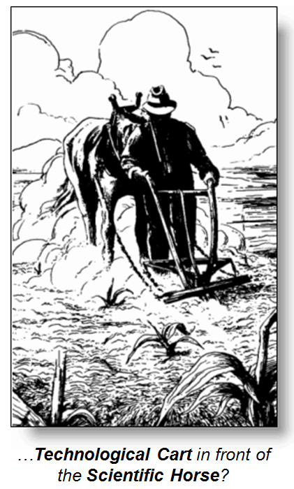
site-specific management. In a sense, technology is ahead of science, sort
of the cart before the horse. A
______________________
 Author’s Note: This column is based on a keynote address for the
Site-Specific Management of Wheat Conference, Denver, Colorado, March 4-5,
1998; a copy of the full text is online at www.innovativegis.com/basis,
select Presentations & Papers.
Author’s Note: This column is based on a keynote address for the
Site-Specific Management of Wheat Conference, Denver, Colorado, March 4-5,
1998; a copy of the full text is online at www.innovativegis.com/basis,
select Presentations & Papers.
The Good, the Bad and the Ugly
Sides of GIS
(GeoWorld, November 2013)
Sometimes GIS-perts imagine geotechnology as
a super hero (“GIS Techymon,” see figure 1) who can
do anything— process data faster than a gigahertz
processor, more powerful than a super computer, able to leap mounds of mapped
data in a single bound and bend hundreds of polylines
with a single click-and-drag—all for truth, justice and all that stuff. With the Spatial Triad for super powers (RS,
GIS, GPS), the legacy of manual mapping has been all but vanquished and
millions upon millions of new users (both human and robotic) rely on GIS Techymon to fill their heads and circuit boards with
valuable insight into “where is what, why, so what and what if” expressions of
spatial patterns and relationships.
In just few decades, vast amounts of spatial data have been collected
and corralled, enabling near instantaneous access to remote sensing images, GPS
navigation, interactive maps, asset management records and geo-queries as a
widely-used “technological” tool. To the
Gen X generation, technology is a mainstay of their lives—geotechnology is
simply another highly useful expression.
A similar but much quieter GIS
revolution as an “analytical” tool (see Author’s Notes 1) has radically changed how foresters, farmers, and city planners
manage their lands; how retail marketers, political forecasters and
epidemiologists “see” spatial relationships in their data sets; how policemen,
generals and political pundits develop tactics for engaging the opposition;
plus thousands of other new paradigms and practices. This growing wealth of sophisticated spatial
models and solutions did not exist a couple of decades
ago, but now they have become indispensible and commonplace parts of
contemporary culture. All is good …or is
it?
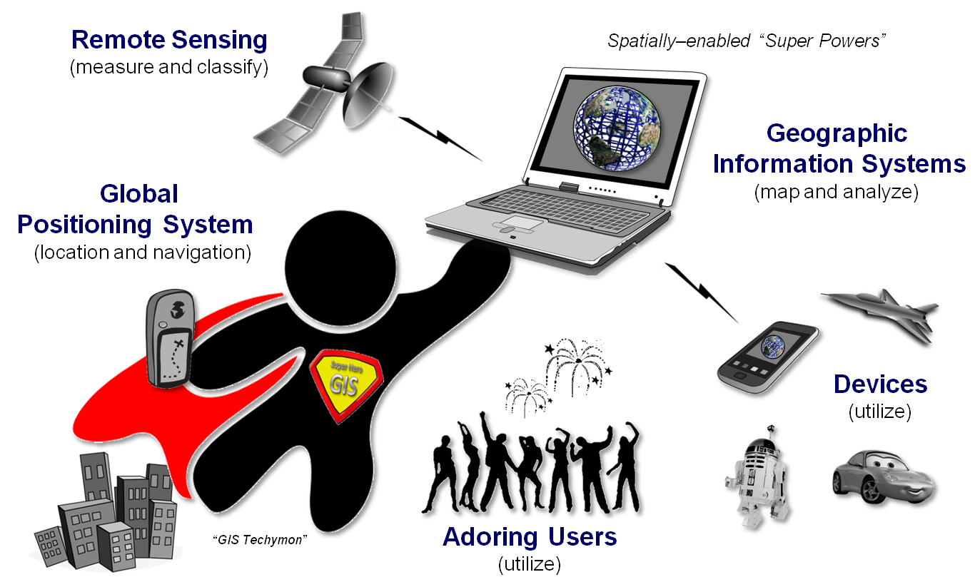
Figure 1. Look up in the data cloud, it’s GIS Techymon to save the
day…all is good (or is it?).
Some fail to see virtue in all
things GIS and actually see the “law of unintended consequences” at play to
expose a darker-side of geotechnology.
Even the best of intentions and ideas can turn bad through unanticipated
effects.
High resolution satellite imagery,
for example, can be used to recognize patterns, map land cover classes and
assess vegetation biomass/vigor throughout the globe—the greater the spatial
detail of the imagery the better the classifications. But in the early 2000s when the satellite
resolution was detailed enough to discern rooftop sun bathers in London the
Internet lit up. It seems zooming in on
an Acacia tree is good but zooming in on people is bad—an appalling violation
of privacy.
Fast forward to today with drone
aircraft tracking people as readily as it tracks an advancing wildfire. Or consider the thousands of in-place and
mobile cameras with sophisticated facial recognition software that shadow
private citizens in addition to criminals and terrorists. Or the concern for data mining of your credit
card swipes, demographic character and life style profile in both space and
time to better market to your needs (good) but at what cost to your privacy
(bad).
Or just last week in my hometown,
a suspect parking database was discovered that has captured license plates
“on-the-fly” for years and can be searched to identify the whereabouts of any
vehicle. The system is good at catching
habitual parking offenders and possibly a bad guy or two, but to many the
technology is seen as a wholesale assault on the privacy of the ordinary good
guy.
The Rorschach ink blot nature of
most technology that flips between good and bad has been debated for
decades. Several years ago I had the
privilege of hosting a Denver University event exploring “Geoslavery
or Cyber-Liberation: Freedom and Privacy in the Information Age” (see Author’s
Note 2). While the panel of experts made
excellent points and provided stimulating discussion, an acceptable balance
that encourages geotechnology’s good side while constraining its bad side was
not struck. The Jekyll and Hyde personality of geotechnology still persists, however it
has been magnified many fold due to its ever-expanding tentacles reaching
further and further into general society.
The collateral damage of
unintended consequences seems to tarnish GIS Techymon’s
image as a classic super hero. However
the purposeful perverse
application of geotechnology is really ugly.
Mark Monmonier’s classic book “How to Lie with Maps” (1996, University Of Chicago Press) reveals how maps can be (and often
must be) distorted to create a readable and understandable map. These cartographic white lies pale in
comparison to the deliberate misrepresentation or misuse of mapped data to
support biased propaganda or hidden agendas.
For example, the top inset in
figure 2 depicts a hypothetical map that rearranges state borders to equally
distribute the population of the United States so each of the
imagined states has1/50th of the total population or about 6 million
people (see Author’s Note 3). This
cartogram is far from an ugly distortion of fact as it effectively conveys
population information in a diagrammatic form that stimulates thought.
The bottom inset addresses the
spatial distribution of population as well.
However, in this case it involves deliberate manipulation of polygon boundaries for
partisan political advantage by combining
census and party affiliation data to “gerrymander” congressional districts (see Author’s Note
4). The drafting
of spindly tentacles and ameba-like pseudopods concentrate the voting power of
one party into as many safe districts as possible and dilute opposition votes
as much as possible. In the opinion of
many political pundits, the GIS-gerrymandered districts are the root-cause of
much of the current bifurcated, dysfunctional and down-right hostile
congressional environment we face.
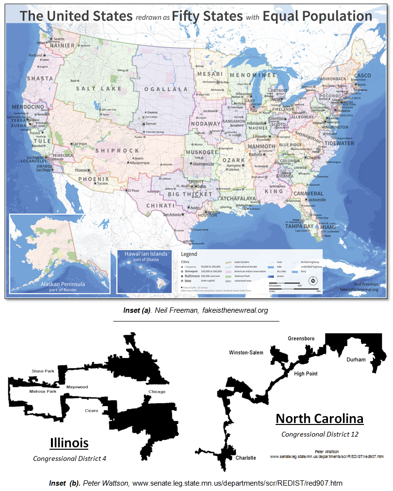
Figure 2. Inset (a) shows a redrawing
of the 50 states forcing equal populations; inset (b) shows examples of deliberate
manipulation of political boundaries for electoral advantage.
Map analysis is very effective in addressing
the gerrymandered spatial optimization problem, regardless of any adverse moral
and political ramifications. It also is
good at efficiently keeping less technologically endowed peoples at bay,
tracking children and the elderly for their own safety, monitoring the
movements of parolees and pedophiles,
fueling information warfare and killing people, and
hundreds of other uses that straddle the moral fence.
GIS is most certainly an agent of good …most
of the time. But it is imperative to
remember that GIS isn’t always good, or always bad, or always ugly. The technological and analytical capabilities
themselves are ethically inert. It is
how they are applied within a social conscience context that determines which
side of GIS surfaces (see Author’s Note 5).
_____________________________
Author’s Notes:
1) See “Simultaneously
Trivializing and Complicating GIS” in the Beyond Mapping Compilation Series at
http://www.innovativegis.com/basis/MapAnalysis/Topic30/Topic30.htm 2) see http://www.innovativegis.com/basis/Present/BridgesGeoslavery/
for panel discussion summary. 3) See “Electoral College Reform (fifty states with
equal population)” at http://fakeisthenewreal.org/reform/. 4) See Beyond
Mapping column on “Narrowing-in on Absurd Gerrymanders” in the Beyond Mapping Compilation
Series at http://www.innovativegis.com/basis/MapAnalysis/Topic25/Topic25.htm
. 5) See “Ethics and GIS: The
Practitioner’s Dilemma” at http://www.spatial.maine.edu/~onsrud/GSDIArchive/gis_ethics.pdf.
Where Do We Go from Here?
(GeoWorld, December 2013)
I have been involved in GIS for over four decades and
can attest that it has matured a lot over that evolutionary/revolutionary
period. In the 25 years of the Beyond
Mapping column, I have attempted to track a good deal of the conceptual,
organizational, procedural, and sometimes disputable issues.
In the 1970s the foundations and fundamental
principles for digital maps took the form of “automated cartography” designed
to replace manual drafting with the cold steel of a pen plotter. In the 1980s we linked these
newfangled digital maps to traditional data base systems to create “spatial
database management systems” that enabled users to easily search for locations
with specific conditions/characteristics, and then display the results in map
form.
The 1990s saw an exponential rise in the use
of geotechnology as Remote Sensing (RS) and the Global Positioning System (GPS)
became fully integrated with GIS— so integrated that GIS World became GeoWorld
to reflect the ever expanding community of users and uses. In addition, map analysis and modeling spawned
a host of new applications, as well as sparking the promise of a dramatic shift
in the historical perspective of “what a map is (and isn’t).”
The 2000s saw the Internet move maps and
mapping from a “down the hall and to the right” specialist’s domain, to
everyone’s desktop, notebook and mobile device.
In today’s high tech environment one can fly-through a virtual reality
rendering of geographic space that was purely science fiction a few decades
ago. Wow!
My ride through GIS’s evolution has been somewhat
akin to Douglas Adams’ Hitchhiker’s Guide to the Galaxy Series. Writing a monthly column on geotechnology
finds resonance in his description of flying— “There is an art, it says, or
rather, a knack to flying. The knack lies in learning how to throw yourself at
the ground and miss.” As GIS evolved,
the twists and turns around each corner were far from obvious, as the emerging
field was buffeted in the combined whirlwinds of technological advances and
societal awakening.
In most cases, geotechnology’s evolution since its
early decades has resulted from outside forces: 1) reflecting macro-changes in
computer science, electrical engineering and general technological advances,
and 2) translating workflows and processes into specialized applications. The results have been a readily accessible
storehouse of digital maps and a wide array of extremely useful and wildly
popular applications. Geotechnology’s
“where is what” data-centric focus has most certainly moved the masses, but has
it moved us closer to a “why, so what, and what if” focus that translates
mapped data into spatial information and understanding?
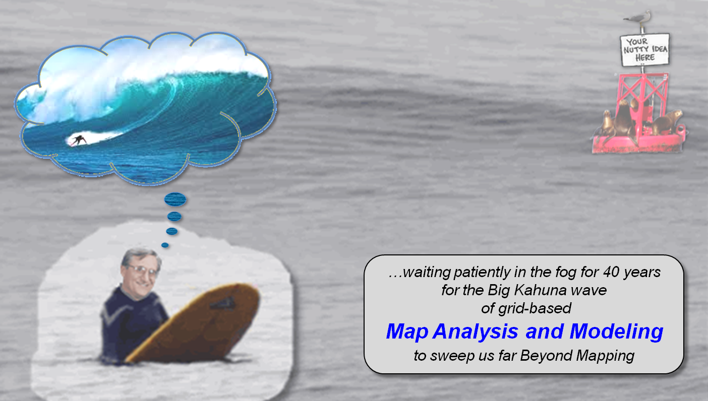
Figure 1. The idea of map variables being
map-ematically evaluated has been around for decades but still not fully
embraced. (I wonder what other nutty
ideas are languishing in the backwaters of geotechnology that have yet to take
form).
While the technological expression of GIS has
skyrocketed, the analytical revolution that was promised still seems
grounded. I have long awaited a Big Kahuna wave of map analysis and modeling (figure 1) to
sweep us well beyond mapping toward an entirely new paradigm of maps, mapping
and mapped data for understanding and directly infusing spatial patterns and
relationships into science and problem-solving.
In the 1970s and 80s my thoughts turned to a “map-ematical” framework for the quantitative analysis of mapped
data (see Author’s Notes 1 and 2). The
suggestion that these data exhibited a “spatial distribution” that was
quantitatively analogous a “numerical distribution” was not well received. The further suggestion that traditional
mathematical and statistical operations could be spatially evaluated was
resoundingly debunked as “disgusting” by the mapping community and “heresy” by
the math/stat community.
In the early years of GIS development, most people
“knew” what a map was (an organized collection of point, line and polygon
spatial objects) and its purpose (display, navigation, and geo-query). To suggest that grid-based maps formed
continuous surfaces defining map variables that could be map-ematically
processed was brash. Couple that
perspective with the rapidly advancing “technological tool” expressions, and
the “analytical tool” capabilities were relegated to the back of the bus.
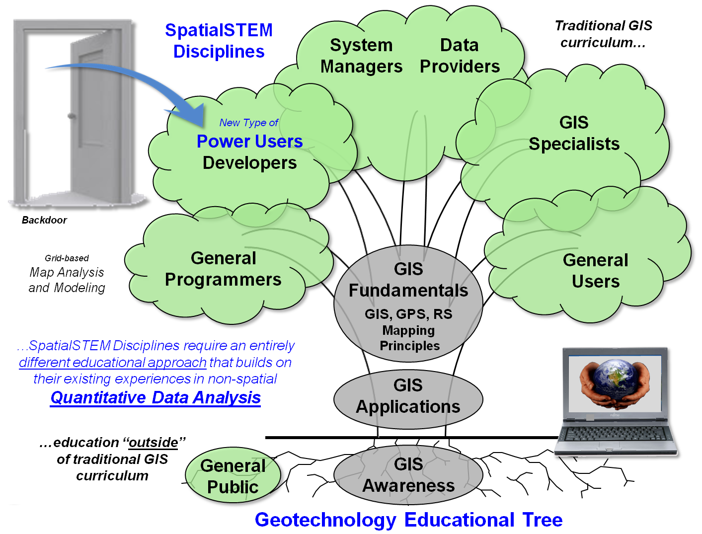
Figure 2. Traditional GIS education does
not adequately address STEM disciplines’ focus on quantitative analysis of
mapped data.
Fast-forward to today and sense the changes in the
wind and sea of thought. Two central
conditions are nudging the GIS oil tanker toward grid-based map analysis and
modeling: 1) the user community is asking “is that all there is to GIS?” (like
Peggy Lee’s classic song but about mapping, display and navigation), and 2) a
building interest in spatialSTEM that is prodding the math/stat community to no
longer ignore spatial patterns and relationships— increasing recognition that
“spatial relationships exist and are quantifiable,” and that “quantitative
analysis of maps is a reality.”
Education will be the catalyst for the next step in
geotechnology’s evolution toward map analysis and modeling. However, traditional GIS curricula and
programs of study (Educational Tree in figure 2) are ill-equipped for the
task. Most STEM students are not
interested in becoming GIS-perts; rather, they want
to employ spatial analysis tools into their scientific explorations—a backdoor
entry as a “Power User.” What we (GIS
communities) need to do is engage the STEM disciplines on their
turf—quantitative data analysis—instead of continually dwelling on the technical
wonders of modern mapping, Internet access, real-time navigation, awesome
displays and elegant underlying theory.
These wonders are tremendously important and
commercially viable aspects of geotechnology, but do not go to the core of the
STEM disciplines (see Author’s Note 3).
Capturing the attention of these folks requires less emphasis on
vector-based approaches involving collections of “discrete map features” for
geoquery of existing map data, and more emphasis on grid-based approaches
involving surface gradients of “continuous map variables” for investigating
relationships and patterns within and among map layers. AKAW!! … surfers cry when they spot a “hugangus”
perfect wave.
However, after 25 years of shuffling along the GIS
path, I have reached my last Beyond Mapping column in GeoWorld …the flickering
torch is ready to be passed to the next generation of GIS enthusiasts. For those looking for an instant replay of
any of the nearly 300 columns, you can access any and all of them through the
Chronological Listing posted at—
http://www.innovativegis.com/basis/MapAnalysis/ChronList/
Also, for the incredibly perseverant, I will be
making a blog post from time to time discussing contemporary issues, approaches
and procedures in light of where we have been (beginning in January 2014)—
I hope some of you will join me on the continuing
journey. Until then …keep on GISing outside the traditional lines.
_____________________________
Author’s Notes:
1) See “An Academic Approach to
Cartographic Modeling in Management of Natural Resources,” 1979 and 2) “A Mathematical Structure for Analyzing Maps,”
1986 …both historical papers posted at www.innovativegis.com/basis/Papers/Online_Papers.htm. 3) See “Topic 30, A Math/Stat Framework for Map Analysis” in the Beyond Mapping Compilation
Series posted at www.innovativegis.com/basis/MapAnalysis/.
(Back to the Table of Contents)