Concepts, Considerations and Procedures in Applying Effective Distance Modeling
Joseph K. Berry1
W. M. Keck Visiting Scholar in Geosciences, Geography,
Principal, Berry & Associates // Spatial Information
Systems (BASIS)
Phone: 970-215-0825 ; Email: jberry@innovativegis.com; Website: www.innovativegis.com
___________________________________
Note:
this paper was presented at the GeoTec Conference,
Abstract
Measuring distance is one
of the oldest and most basic map analysis techniques. However, the traditional concept of distance
as “the shortest straight-line between two points” reflects our paper map
legacy more than the reality of movement.
While a straight-line route may indicate the distance “as the crow
flies,” it offers little information for a walking crow, customers driving to
your store, water flow over a terrain surface or other real world
situations. Effective distance extends
the concept of Distance to one of Proximity by relaxing the limitation of
“…between two points” by simultaneously considering measurements among sets of
point, line and polygon features. The
concept is further extended to one of Movement
throughout geographic space by considering relative and absolute barriers that
relax the limitation of “…straight line…”
Within contemporary
Introduction
Measuring distance is one of the most basic map analysis techniques. Historically, distance is defined as the shortest straight-line between two points. While this three-part definition is both easily conceptualized and implemented with a ruler, it is frequently insufficient for decision-making. A straight-line route might indicate the distance “as the crow flies,” but offer little information for the walking crow or other flightless creature. It is equally important to most travelers to have the measurement of distance expressed in more relevant terms, such as time or cost.
The limitation of a map analysis approach is not so much in the concept of distance measurement, but in its implementation. Any measurement system requires two components— a standard unit and a procedure for measurement. Using a ruler, the “unit” is the smallest hatching along its edge and the “procedure” is the line implied by the straightedge. In effect, the ruler represents just one row of a grid implied to cover the entire map. You just position the grid such that it aligns with the two points you want measured and count the squares (top portion of figure 1). To measure another distance you merely realign the implied grid and count again.
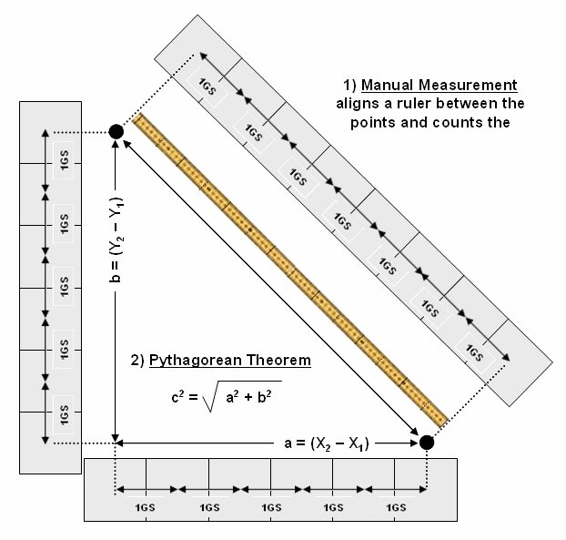
Figure
1. Both Manual Measurement and the
Pythagorean Theorem use grid spaces as the fundamental units for determining
the distance between two points.
In
a
Extending the Concept of Distance to
Proximity
Proximity establishes the distance to all locations surrounding a point— the set of shortest straight-lines among groups of points. Rather than sequentially computing the distance between pairs of locations, concentric equidistance zones are established around a location or set of locations (figure 2). This procedure is similar to the wave pattern generated when a rock is thrown into a still pond. Each ring indicates one “unit farther away”— increasing distance as the wave moves away. Another way to conceptualize the process is nailing one end of a ruler at a point and spinning it around. The result is a series of “data zones” emanating from a location and aligning with the ruler’s tic marks.
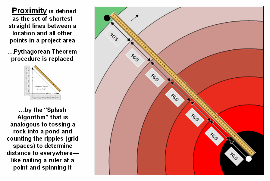
Figure
2. Proximity identifies the set of
shortest straight-lines among groups of points (distance zones).
However, nothing says proximity must be measured from a single point. A more complex proximity map would be generated if, for example, all locations with houses (set of points) are simultaneously considered target locations (right side of figure 3). In effect, the procedure is like throwing a handful of rocks into pond. Each set of concentric rings grows until the wave fronts from other locations meet; then they stop. The result is a map indicating the shortest straight-line distance to the nearest target area (house) for each non-target area. In the figure, the red tones indicate locations that are close to a house, while the green tones identify areas that are far from a house.
Figure
3. Proximity surfaces can be generated
for groups of points, lines or polygons identifying the shortest distance from
all location to the closest occurrence.
In a similar fashion, a proximity map to roads is generated by establishing data zones emanating from the road network—sort of like tossing a wire frame into a pond to generate a concentric pattern of ripples (middle portion of figure 3). The same result is generated for a set of areal features, such as sensitive habitat parcels (right side of figure 3).
It is important to note that proximity is not the same as a buffer. A buffer is a discrete spatial object that identifies areas that are within a specified distance of map feature; all locations within a buffer are considered the same. Proximity is a continuous surface that identifies the distance to a map feature(s) for every location in a project area. It forms a gradient of distances away composed of many map values; not a single spatial object with one characteristic distance away.
The 3D plots of the proximity surfaces in figure 3 show detailed gradient data and are termed accumulated surfaces. They contain increasing distance values from the target point, line or area locations displayed as colors from red (close) to green (far). The starting features are the lowest locations (black= 0) with hillsides of increasing distance and forming ridges that are equidistant from starting locations.
Calculating Simple Proximity
The previous section established that proximity is measured by a series of propagating rings emanating from a starting location—splash algorithm. Since the reference grid is a set of square grid cells, the rings are formed by concentric sets of cells. In figure 4, the first “ring” is formed by the three cells adjoining the starting cell in the lower-right corner. The top and side cells represent orthogonal movement while upper-left one is diagonal. The assigned distance of the steps reflect the type of movement—orthogonal equals 1.000 and diagonal equals 1.414.
As the rings progress, 1.000 and 1.414 are added to the previous accumulated distances resulting in a matrix of proximity values. The value 7.01 in the extreme upper-left corner is derived by adding 1.414 for five successive rings (all diagonal steps). The other two corners are derived by adding 1.000 five times (all orthogonal steps). In these cases, the effective proximity procedure results in the same distance as calculated by the Pythagorean Theorem.
Figure
4. Simple proximity is generated by
summing a series of orthogonal and diagonal steps emanating from a starting
location.
Reaching other locations involve combinations of orthogonal and diagonal steps. For example, the other location in the figure uses three orthogonal and then two diagonal steps to establish an accumulated distance value of 5.828. The Pythagorean calculation for same location is 5.385. The difference (5.828 – 5.385= .443/5.385= 8%) is due to the relatively chunky reference grid and the restriction to grid cell movements.
Grid-based proximity measurements tend to overstate true distances for off-orthogonal/diagonal locations. However, the error becomes minimal with distance and use of smaller grids. And the utility of the added information in a proximity surface often outweighs the lack of absolute precision of simple distance measurement.
Figure
5. Simple distance rings advance by
summing 1.000 or 1.414 grid space movements and retaining the minimal
accumulated distance of the possible paths.
Figure 5 shows the calculation details for the remaining rings. For example, the larger inset on the left side of the figure shows ring 1 advancing into the second ring. All forward movements from the cells forming the ring into their adjacent cells are considered. Note the multiple paths that can reach individual cells. For example, movement into the top-right corner cell can be an orthogonal step from the 1.000 cell for an accumulated distance of 2.000. Or it can be reached by a diagonal step from the 1.414 cell for an accumulated distance of 2.828. The smaller value is stored in compliance with the idea that distance implies “shortest.” If the spatial resolution of the analysis grid is 300m then the ground distance is 2.000 * 300m/gridCell= 600m.
In a similar fashion, successive ring movements are calculated, added to the previous ring’s stored values, and the smallest of the potential distance values being stored. The distance waves rapidly propagate throughout the project area with the shortest distance to the starting location being assigned at every location.
If more than one starting location is identified, the proximity surface for the next starter is calculated in a similar fashion. At this stage every location in the project area has two proximity values—the current proximity value and the most recent one (figure 6). The two surfaces are compared and the smallest value is retained for each location—distance to closest starter location. The process is repeated until all of the starter locations representing sets of points, lines or areas have been evaluated.
Figure
6. Proximity surfaces are compared and
the smallest value is retained to identify the distance to the closest starter
location.
While the computation is overwhelming for humans, the repetitive nature of adding constants and testing for smallest values is a piece of cake for computers (millions of iterations in a few seconds). More importantly, the procedure enables a whole new way of representing relationships in spatial context involving “effective distance” that responds to realistic differences in the characteristics and conditions of movement throughout geographic space.
Extending the Concept of Simple Proximity to Movement
In many applications, however, the shortest route between two locations might not always be a straight-line (or even a slightly wiggling set of grid steps). And even if it is straight, its geographic length may not always reflect a traditional measure of distance. Rather, distance in these applications is best defined in terms of “movement” expressed as travel-time, cost or energy that is consumed at rates that vary over time and space. Distance modifying effects involve weights and/or barriers— concepts that imply the relative ease of movement through geographic space might not always constant.
Figure 7 illustrates one of the effects of distance being affected by a movement characteristic weight. The left-side of the figure shows the simple proximity map generated when both starting locations are considered to have the same characteristics or influence. Note that the midpoint (dark green) aligns with the perpendicular bisector of the line connecting the two points and confirms a plane geometry principle you learned in junior high school.
Figure
7. Weighting factors based on the
characteristics of movement can affect relative distance, such as in Gravity
Modeling where some starting locations exert more influence than others.
The right-side of the figure, on the other hand, depicts effective proximity where the two starting locations have different characteristics. For example, one store might be considered more popular and a “bigger draw” than another (Gravity Modeling). Or in old geometry terms, the person starting at S1 hikes twice as fast as the individual starting at S2— the weighted bisector identifies where they would meet. Other examples of weights include attrition where movement changes with time (e.g., hiker fatigue) and change in mode (drive a vehicle as far as possible then hike into the off-road areas).
In addition to weights that reflect characteristics of the movement itself, effective proximity responds to intervening conditions or barriers. There are two types of barriers that are identified by their effects— absolute and relative. Absolute barriers are those completely restricting movement and therefore imply an infinite distance between the points they separate. A river might be regarded as an absolute barrier to a non-swimmer. To a swimmer or a boater, however, the same river might be regarded as a relative barrier identifying areas that are passable, but only at a cost which can be equated to an increase in geographical distance. For example, it might take five times longer to row a hundred meters than to walk that same distance.
In the conceptual framework of tossing a rock into a pond, the waves can crash and dissipate against a jetty extending into the pond (absolute barrier; no movement through the grid spaces). Or they can proceed, but at a reduced wavelength through an oil slick (relative barrier; higher cost of movement through the grid spaces). The waves move both around the jetty and through the oil slick with the ones reaching each location first identifying the set of shortest, but not necessarily straight-lines among groups of points.
The
shortest routes respecting these barriers are often twisted paths around and
through the barriers. The
Figure
8. Effective Proximity surfaces consider
the characteristics and conditions of movement throughout a project area.
The point features in the left inset respond to treating flowing water as an absolute barrier to movement. Note that the distance to the nearest house is very large in the center-right portion of the project area (green) although there is a large cluster of houses just to the north. Since the water feature can’t be crossed, the closest houses are a long distance to the south.
Terrain steepness is used in the middle inset to illustrate the effects of a relative barrier. Increasing slope is coded into a friction map of increasing impedance values that make movement through steep grid cells effectively farther away than movement through gently sloped locations. Both absolute and relative barriers are applied in determining effective proximity sensitive areas in the right inset.
Compare these results with those in figure 3 and note the dramatic differences between the concept of distance “as the crow flies” (simple proximity) and “as the crow walks” (effective proximity). In many practical applications, the assumption that all movement occurs in straight lines disregards reality. When traveling by trains, planes, automobiles, and feet there are plenty of bends, twists, accelerations and decelerations due to characteristics (weights) and conditions (barriers) of the movement.
Figure 9 illustrates how the splash algorithm propagates distance waves to generate an effective proximity surface. The Friction Map locates the absolute (blue/water) and relative (light blue= gentle/easy through red= steep/hard) barriers. As the distance wave encounters the barriers their effects on movement are incorporated and distort the symmetric pattern of simple proximity waves. The result identifies the “shortest, but not necessarily straight” distance connecting the starting location with all other locations in a project area.
Figure
9. Effective Distance waves are distorted as they encounter absolute and
relative barriers, advancing faster under easy conditions and slower in
difficult areas.
Note that the absolute barrier locations (blue) are set to infinitely far away and appear as pillars in the 3-D display of the final proximity surface. As with simple proximity, the effective distance values form a bowl-like surface with the starting location at the lowest point (zero away from itself) and then ever-increasing distances away (upward slope). With effective proximity, however, the bowl is not symmetrical and is warped with bumps and ridges that reflect intervening conditions— the greater the impedance the greater the upward slope of the bowl. In addition, there can never be a depression as that would indicate a location that is closer to the starting location than everywhere around it. Such a situation would violate the ever-increasing concentric rings theory and is impossible except on Star Trek where Spock and the Captain de-materialize then reappear somewhere else without physically passing through the intervening locations.
Calculating Effective Proximity
Basic to this expanded view of distance is conceptualizing the measurement process as waves radiating from a location(s)— analogous to the ripples caused by tossing a rock into a pond. As the wave front moves through space, it first checks to see if a potential “step” is passable (absolute barrier locations are not). If not passable, the distance is set to infinitely far away. If passable, the wave front moves there and incurs the “cost” of such a movement identified on the Friction Map (relative barrier values of impedance). As the wave proceeds, all possible paths are considered and the shortest distance assigned (least total impedance from the starting point).
Figure
10. Effective proximity is generated by
summing a series of steps that reflect the characteristics and conditions of
moving through geographic space.
Figure 10 shows the effective proximity values for a small portion of the results forming the surface shown in figure 9. Manual Measurement, Pythagorean Theorem and Simple Proximity all report that the geographic distance to the location in the upper-right corner is 5.071 * 300meters/gridCell= 1521 meters (see figures 1 and 4). But this simple geometric measure assumes a straight-line connection that crosses extremely high impedance values, as well as absolute barrier locations—an infeasible route that results in exhaustion and possibly death of a walking crow.
The shortest path respecting absolute and relative barriers is shown as first sweeping to the left and then passing around the barrier on the right side. This counter-intuitive route is formed by summing the series of shortest steps at each juncture. The first step away from the starting location is toward the lowest friction and is computed as the impedance value times the type of step for 3.00 *1.000= 3.00. The next step is considerably more difficult at 5.00 * 1.414= 7.07 and when added to the previous step’s value yields a total effective distance of 10.07. The process of determining the shortest step distance and adding it to the previous distance is repeated over and over to generate the final accumulated distance of the route.
It is important to note that the resulting value of 49.70 can’t be directly compared to the 507.1 meters geometric value. Effective proximity is like applying a rubber ruler that expands and contracts as different movement conditions reflected in the Friction Map are encountered. However, the proximity values do establish a relative scale of distance and it is valid to interpret that the 49.7 location is nearly five times farther away than the location containing the 10.07 value.
If the Friction Map is calibrated in terms of a standard measure of movement, such as time, the results reflect that measure. For example, if the base friction unit was 1-minute to cross a grid cell the location would be 49.71 minutes away from the starting location. What has changed isn’t the fundamental concept of distance but it has been extended to consider real-world characteristics and conditions of movement that can be translated directly into decision contexts, such as how long will it take to hike from “my cabin to any location” in a project area. In addition, the effective proximity surface contains the information for delineating the shortest route to anywhere—simply retrace to wave front movement that got there first by taking the steepest downhill path over the accumulation surface.
Figure
11. Effective distance rings advance by
summing the friction factors times the type of grid space movements and retaining
the minimal accumulated distance of the possible paths.
The calculation of effective distance is similar to that of simple proximity, just a whole lot more complicated. Figure 11 shows the set of movement possibilities for advancing from the first ring to the second ring. Simple proximity only considers forward movement whereas effective proximity considers all possible steps (both forward and backward) and the impedance associated with each potential move.
For example, movement into the top-right corner cell can be an orthogonal step times the friction value (1.000 * 6.00) from the 18.00 cell for an accumulated distance of 24.00. Or it can be reached by a diagonal step times the friction value (1.414 * 6.00) from the 19.00 cell for an accumulated distance of 30.48. The smaller value is stored in compliance with the idea that distance implies “shortest.” The calculations in the blue panels show locations where a forward step from ring 1 is the shortest, whereas the yellow panels show locations where backward steps from ring 2 are shorter.
The explicit procedure for calculating effective distance in the example involves:
Step 1) multiplying the
friction value for a step
Step 2) times the type of
step (1.000 or 1.414)
Step 3) plus the current
accumulated distance
Step 4) testing for the
smallest value, and
Step 5) storing the
minimum solution if less than any previously stored value.
Extending the procedure to consider movement characteristics merely introduces an additional step at the beginning—multiplying the relative weight of the starter.
Figure 12. Effective proximity surfaces are computed respecting movement weights and impedances then compared and the smallest value is retained to identify the distance to the closest starter location.
The complete procedure for determining effective proximity from two or more starting locations is graphically portrayed in figure 12. Proximity values are calculated from one location then another and stored in two matrices. The values are compared on a cell-by-cell basis and the shortest value is retained for each instance. The “calculate then compare” process is repeated for other starting locations with the working matrix ultimately containing the shortest distance values, regardless which starter location is closest. Piece-of-cake for a computer.
Conclusion
While the computations of simple and effective proximity might appear complex, once coded they are easily and quickly performed by modern computers. In addition, there is a rapidly growing wealth of digital data describing conditions that impact movement in the real world. What seems to be the impediment for use of this new way of expressing distance as proximity and movement lies in the experience base of potential users. Our paper map legacy suggests that the “shortest straight line between two points” is the only way to investigate spatial context relationships and anything else is disgusting (or at least uncomfortable).
This
limited perspective has lead most contemporary
___________________________
Additional References
Additional
discussion of distance, proximity, movement and related measurements in
http://www.innovativegis.com/basis/
See Map Analysis Topics…
¾ Topic 25, Calculating Effective Proximity
¾ Topic 20, Surface Flow Modeling
¾ Topic 19, Routing and Optimal Paths
¾ Topic 17, Applying Surface Analysis
¾ Topic 15, Deriving and Using Visual Exposure Maps
¾ Topic 14, Deriving and Using Travel-Time Maps
¾ Topic 13, Creating Variable-Width Buffers
¾ Topic 6, Analyzing In-Store Shopping Patterns
¾ Topic 5, Analyzing Accumulation Surfaces
About the Author
 Joseph K. Berry is a leading
consultant and educator in the application of Geographic Information Systems (
Joseph K. Berry is a leading
consultant and educator in the application of Geographic Information Systems (