GeoWorld Articles
|
Further Understanding Spatial Patterns and Relationships ( |

Feature
article for GeoWorld, March 2006, Vol. 19, No. 3, pgs. 22-25
<Click here>
right-click for a printer-friendly version of this paper (.pdf).
Beyond Location, Location, Location: Retail
Sales Competition Analysis
by Joseph K,
Introduction
For years businesses have generally ignored
spatial relationships in data analysis. While
common sense considers “location, location, location” a cornerstone of
business, traditional analysis procedures force spatial information, such as
customer location, to be aggregated into large generalized reporting units. Pockets of sales on one side of a trade area
are not differentiated from those on another side.
Geo-Business
describes an emerging discipline that uses Geographic Information Systems (
Site
location is an early example of extending these basic mapping capabilities to
map analysis. The application uses
The
latter two of these emerging Geo-business applications, Competition Analysis
and Predictive Modeling, serve as the focus of this paper. The discussion summarizes the primary steps
involved in generating predicted sales maps for various products. The approach
is based on competitor locations to model relative travel-time advantage and
existing customer data to model sales patterns and travel-time
sensitivity. While the experience described
is the result of an ambitious prototype model involving a large metropolitan
area and tens of thousands of customer records, the graphics shown have been
altered and the details of implementation and results are curtailed.
Deriving Travel Time
Maps
Most
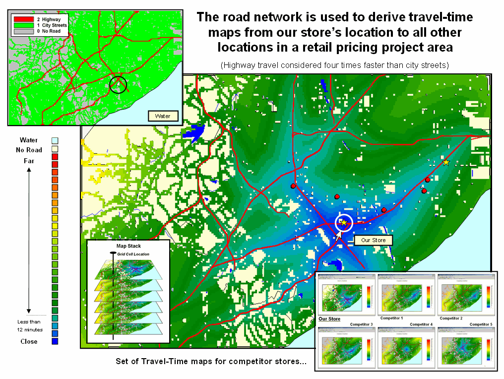
Figure 1.
Grid-based travel time analysis involves calculating effective proximity as a
series of propagating waves that respond to various speeds along the road map
resulting in access zones from close (blue) to far (red).
For
example, the extent of project area shown in figure 1 is an 18 by 23 mile swath
of a major metropolitan area capturing hundreds of thousands of
residences. The inset in the upper left
corner shows primary and secondary roads defining an analysis frame of the area
comprised of four-hectare grid cells within a matrix of 228 columns by 153 rows
(34,884 sample locations). This spatial
resolution is appropriate for strategic-level competition analysis; however a
higher resolution is easily imposed by specifying a smaller grid size during
the vector to raster conversion of the road map.
The
large map in the center depicts the calculated travel time from “Our Store” to
all other grid locations in the project area.
The blue tones identify grid cells that are less than twelve minutes
away assuming travel on the highways is four times faster than on city
streets. Note the star-like pattern
elongated around the highways and progressing to the farthest locations (warmer
tones). Competitor locations are
indicated by the red dots. The tan areas are parks and natural or industrial
locations not served by the road network.
The
grid-based procedure is not as exacting as point-to-point solutions as it
ignores one-way streets, left-turn waits, and other navigational factors;
however the relative access surface it generates is appropriate for competition
analysis (see Authors’ Note 1). In a similar manner, competitor stores are
identified and the set of their travel time surfaces forms a geo-registered map
stack supporting analysis.
Determining Relative
Gain for Stores
The
travel-time surfaces summarize relative customer access to our store and
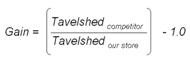
competitor stores for all grid locations in the trade area. Figure 2 shows 2D and 3D displays of the
surfaces for our store and competitor #4.
Note that a travel-time surface is shaped like a bowl with the bottom of
the bowl at the store’s location (map value= zero away) and the walls formed by
increasingly larger travel-time values.
For any given location, the two travel-time values for a pair of
surfaces can be easily retrieved and compared by subtracting. In the example, the subject location in the
figure is 17.2 minutes (34.4 cells away * .05 minutes/cell) from our store
versus 42.1 minutes for competitor #4 store—a significant 24.9 minute advantage
for our store.
A
more useful Travel-Time Gain factor for modeling can be derived by evaluating
the grid-math equation,
for
two travel-time maps at every grid location in the project area. The result is a map indicating the relative
cost of visitation choices between the two stores for every grid location. A Gain of less than 1.0 indicates the
competition has an advantage with larger values indicating increasing advantage
for our store. For example, a value of
2.0 indicates that there is a 200%
lower cost of visitation to our store over the competition.
Figure
2. The Travel-time value stored at each grid
location specifies how far away it is from a store—location 103c, 86r is 17.2
minutes away from Our Store and 42.1 minutes away from Competitor #4 Store.
The Gain factor is a stable, continuous variable
encapsulating travel-time differences that is suitable for mathematical
modeling (see Author’s Note 3). A Gain calculation summarizing travel-time
advantages between our store and a competitor store is made for each cell in
the project area. These Gain
calculations are used as input to the sales prediction models reported
below.
Overview of Processing
Steps
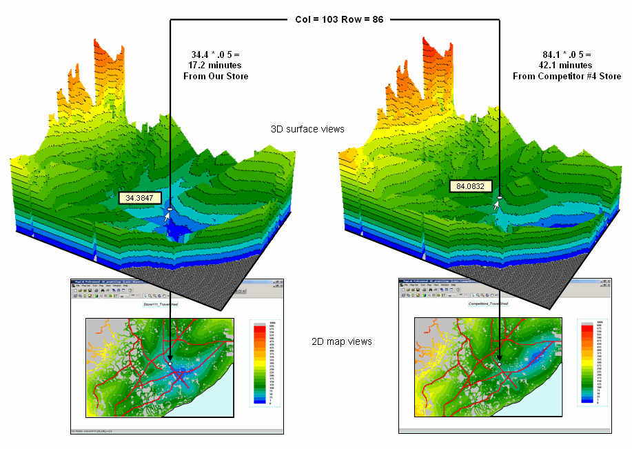
Figure 3a summarizes the
spatial modeling steps involved in competition analysis. The first and second steps use grid-based map
analysis procedures to construct travel-time maps for all stores of interest
within the market area. The third step
generates mapped data of the relative gain for our store and each of the
competitor stores.
Figure 3a.
Spatial Modeling steps derive the relative travel time relationships for our
store and each of the competitor stores for every location in the project area
and links this information to customer records.
Critical throughout these
steps is the use of geo-coding through address-matching to map each person in
the region to a discrete grid cell based on latitude and longitude of their
home street address. This provides a
universal key for transferring and integrating spatial information of
Travel-Time and Gain to and from a database of non-spatial customer information
that can be summed, averaged, counted or otherwise described for each grid cell
and surrounding groups of cells defining town boundaries or sales
districts.
The
Travel-Time Gain data is the cornerstone of competition analysis. It provides a consistent measure of store
competition that can be used in data mining along with traditional non-spatial
variables such as customer sales activity, demographics, economics, life-style and
life-stage information. This link
between spatial and non-spatial information supports the development of
predictive models that consider detailed “location, location, location”
information within traditional data mining procedures.
For the predictive
modeling, we used a regression approached using a specialized data mining
technology, KXEN K2R, based on Vapnik Statistical Learning theory (see
Authors’ Note 3). This commercially
available technology is similar to linear or logistic regression except that
the convergence algorithms are not based on least-squares techniques. A main
advantage is that non-linearity in the continuous input variables are
represented by piece-wise linear terms, rendering hand transforms to add power
terms (e.g. y = a + bx + cx2) unnecessary.
The tool also can
automatically detect and handle multi-colinearity and works with ordinal and
nominal input data as well as continuous variables. It is capable of building excellent models
from very large data sets, with thousands of columns and millions of rows of
data in a single step. These very large
models can be automatically reduced to the minimal set of independent variables
in a second modeling pass where information contribution criteria are applied
to eliminate variables from the equation, in a manner loosely analogous to
stepwise linear regression.
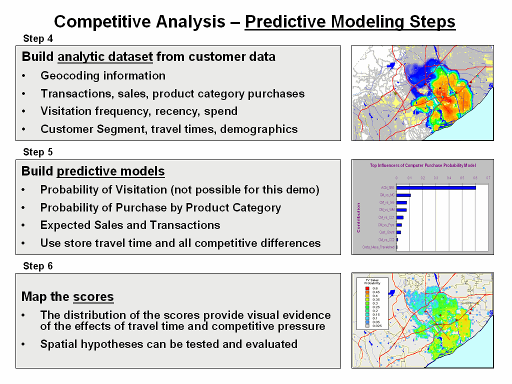
Figure
3b. Predictive Modeling steps use spatial
data mining procedures for relating spatial and non-spatial factors to sales
data to derive maps of expected sales for various products.
Figure 3b summarizes the
predictive modeling steps involved in competition analysis of retail data. For the examples in this paper, a dataset was
developed containing sales history for more than 80,000 customers in the
trading area. Using latitude and longitude of each street address, customers
were geo-coded to the map and the grid row and column coordinates assigned by
membership within the latitude and longitude coordinates of a grid cell. Thus each consumer was assigned to a grid
cell location, for which the travel-times to all stores in the region were
known. The regression hypothesis was
that sales would be predictable by characteristics of the customer in
combination with the travel-time variables.
A summary of the dataset
records used to develop the predictive models is shown in Table 1. The first five entries identify a customer
and their derived grid cell location in the analysis grid. The next several entries are derived factors
including non-spatial Customer Segment assignment and spatial Travel-time and
Gain factors that are used as drivers by the prediction model. The remaining entries are target variables.
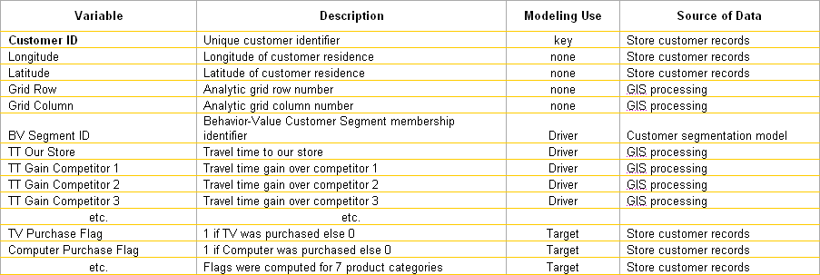
Table
1. Description of record types in the
combined spatial and non-spatial data set for predictive modeling.
In Step 5 of figure 3b, a
series of mathematical models are built that predict the probability of
purchase for each product category under analysis. This provides a set of model scores for each
customer in the region. Non-customers
could be scored with these models, but that was beyond the scope of the
demonstration project. Since a number of
customers could be found in most grid cells, the scores were averaged to
provide an estimate of the likelihood that a person from each grid cell would
travel to our store to purchase one of the analyzed products.
Specifically, purchase
probabilities for seven product categories were modeled for each grid
cell. The final step in the process
simply maps the scores for visual analysis or subsequent analysis, such
targeted marketing.
Example Results
The
upper right inset in figure 4 summarizes the processing flow for mapping the
probability of purchase. An analysis
dataset is constructed containing customer data, geographic location and
derived spatial and non-spatial variables used in predictive modeling. The probability of purchasing a specified
product is derived for each customer and the individual probabilities in a grid
cell are averaged, then the resulting map is displayed.
Note
in the example that the non-spatial summaries identifies that the most
important variable in the model is the derived Customer Segmentation
grouping. The next most import variable
is the Gain Factor for competitor #5, identifying that for Computer Sales this
store represents our greatest competition.
This is somewhat counter intuitive as the map of computer sales
probability shows this store fairly far away and in an area of only moderate TV
sales probability. It suggests that
customers are somewhat more elastic toward travel for computer purchases than
Phone or TV purchases as shown in the two smaller maps on the right.
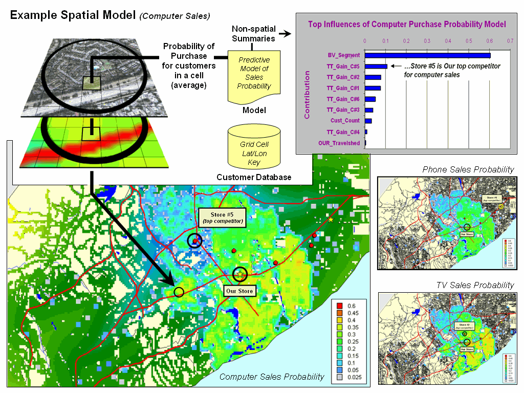
Figure
4. Mapping the results of the prediction
models provides insight into the level and geographic distribution of probable
sales, as well as the competitor environment.
The
information on the level of probable sales, its distribution throughout the
trade area and competitor environment can be invaluable in marketing decisions
and developing strategies for product mix and sales emphasis.
Conclusion
Several
summary and concluding points can be made—
-
Historically
spatial information has been ignored or at least aggregated to effectively
non-spatial levels
-
Grid-based
map analysis provides a consistent base unit (grid cell) for calculating
spatial context and facilitating the linkage of
-
Travel-time
and its derivative Gain Factor summarize the relative access cost for customers
between stores
-
Spatial Modeling provides a new dimension to
customer understanding
-
Sales can be related to Competitors as well as
Customer Segments and groups
-
New customer acquisition targeting can take spatial
factors into account
-
Specific product categories have very different
spatial distributions
-
Competitive factors can be discovered and managed
-
Sales potential modeling/mapping identifies
opportunities by product supporting target marketing, and
-
Store placement can leveraged through better
understanding of competitive and customer positioning.
“Location,
location, location” is a cornerstone of the business environment. The potential of the convergence of spatial
and non-spatial information in data mining and predictive modeling is
great. As business interests and
_____________________________
Authors’
Notes:
1) For more information
about travel-time calculations and applications in geo-business see www.innovativegis.com/basis/,
select the Map Analysis online book, Topic 14, “Deriving and Using Travel-time
Maps.”
2) For some purposes, it might be useful to
transform the Gain equation to a logarithmic form (log(Gain)) that would
linearize the function and perhaps better represent areas where competitor has
an advantage.
3) For more information
on the Knowledge Extraction Engines (Kxen) spatial data mining technology used
in developing the predictive models see www.kxen.com/news/2003/12/veolia_water_systems.php
__________________________________
Joseph K,
Keck Scholar in
Geosciences,
Kenneth L. Reed
Senior Director of
Business Analytics, LowerMyBills.com