Incorporating Grid-based Map Analysis into
GIS Curricula
Joseph K. Berry1
W. M. Keck Visiting Scholar
in Geosciences,
Principal, Berry &
Associates // Spatial Information Systems (BASIS)
Phone:
970-215-0825; Email: jberry@innovativegis.com;
Website: www.innovativegis.com
(Note:
this paper was presented at the 2007 GeoTec Conference, Calgary, Alberta,
Canada, May 14-17; click here for .pdf
version)
Abstract
Popularity of inexpensive and
easy-to-use desktop mapping systems has fueled introductory GIS course
offerings in a variety of disciplines on most campuses. Textbooks and supplemental teaching materials
support basic concepts and procedures, such as data issues, thematic mapping,
geo-query and display. However, the bulk
of the teaching materials focus on vector data processing and applications, with
none or minimal reference to grid-based map analysis. This paper describes a comprehensive set of
materials for instructors and students providing hands-on exposure to the
concepts, capabilities and considerations in grid-based map analysis and modeling.
Instructional
Materials (available June, 2007)
The Instructor CD for Grid-based
Map Analysis contains a comprehensive set of instructional materials
supporting a variety of workshops and courses including syllabus, PowerPoint lectures,
exercises, databases, and study/exam questions with answers. The topics covered include data structure,
display types, vector-raster data exchange, analytical operations and GIS
modeling. The instructional materials
are available for US$45 plus shipping and handling charges
(for more information or to order contact the author at jberry@innovativegis.com).

The materials extend the discussions
in the Map Analysis book (Berry,
2007; GeoTec Media, $45.20 which includes S&H; see www.geoplace.com/books/MapAnalysis) and its MapCalc companion
software (see www.redhensystems.com, select Productsà MapCalc; a GeoWorld Review of the MapCalc software is
posted at www.innovativegis.com/basis/present/GW01_MCreview/GW_JUN01_mapcalcReview.htm).
The lecture sets and hands-on
exercises focus on two broad groups of grid-based map analysis operations. The Spatial Analysis operations
investigate the “contextual” relationships in mapped data and are divided into
logical classes based on processing similarities—Reclassifying Maps, Overlaying
Maps, Measuring Distance and
Connectivity, and Neighborhood
Summary. Numerous examples of GIS
models are included and students are encouraged to encode local data and
formulate their own models.
The Spatial Statistics
experience focuses on the “numerical” relationships and is divided into two
classes of operations—Surface Modeling
involving spatial interpolation of point data into continuous geographic
distributions and Spatial Data Mining
investigating numerical relationships within and among mapped data to include
predictive modeling.
Much of the material was
developed and originally presented at the
Background
Courses in Geographic
Information Systems (GIS) technology are proliferating on campuses. While GIS used to be the domain of geography
departments, it has diffused into application disciplines ranging from forestry
to business, engineering, law enforcement, public health and a multitude of
other departments. A major factor
fueling the expansion is inexpensive and user-friendly desktop mapping software.
These vector-based systems
are ideal for learning the fundamentals of mapping and spatial database
management. The educational experience
with desktop mapping provides an excellent entry into GIS and hands-on experience
in applying the basic concepts. An
increasing number of resources tailored to specific application areas are
available. The datasets and structured
exercises provide meaningful learning experiences for a wide range of students.
Basic thematic mapping and
geo-query, however, only address a portion of GIS capabilities and grid-based
map analysis hasn’t received the same attention in most academic programs. This condition often is attributed to less
familiar analysis techniques that are outside manual mapping experiences and,
until recently, involved complex software running on expensive hardware
platforms and requiring specialized programming knowledge. The result is that through exposure to
grid-based analysis capabilities rarely occurs in introductory courses.
Grid-based maps represent a
different paradigm of geographic space.
Whereas traditional vector maps emphasize “precise placement of physical
features,” grid maps seek to “statistically characterize continuous space in
both real and cognitive terms.” The
tools for mapping of database attributes are extended to analysis of spatial
relationships. The remainder of this
paper describes some of the basic concepts, considerations and procedures in
grid-based data handling and analysis operations.
Grid-Based Analysis Frame
Vector-based systems identify
three basic map features that comprise all maps—points, lines and
polygons. These features are
suitable for characterizing discrete spatial objects, such as light poles,
streets and property boundaries.
However, continuous gradients, such as an elevation surface or a
proximity map are poorly represented as contour lines that generalize detailed
data into a set of intervals used for display.
The introduction of a
grid-analysis frame provides a framework for storage and processing of a fourth
basic map feature—a surface—as well as supporting a host of new analysis
operations by treating geographic space as a informally sampled continuum. Its base spatial unit is a “cell” defined by
the column and row coordinates of an imaginary grid superimposed over an area.
The grid cell and is used to statistically characterize:
-
points as individual cells,
-
lines as connected sets of cells,
-
polygons as all cells identifying the edge and interior of
discrete parcels, and
-
a surface as all of the cells within a project area with a
value assigned to each that indicates the presence by feature type (discrete
object) or the relative variable response (continuous gradient).
The top-left portion of
figure 2 shows an elevation surface displayed as a traditional contour map, a
superimposed analysis frame and a 2-D grid map.
The highlighted location depicts the elevation value (1,635 feet) stored
at one of the grid locations. The pop-up
table at the lower-right shows the values stored on other map layers for a
selected location. As the cursor is
moved, the “drill-down” of values for different locations are instantly
updated.
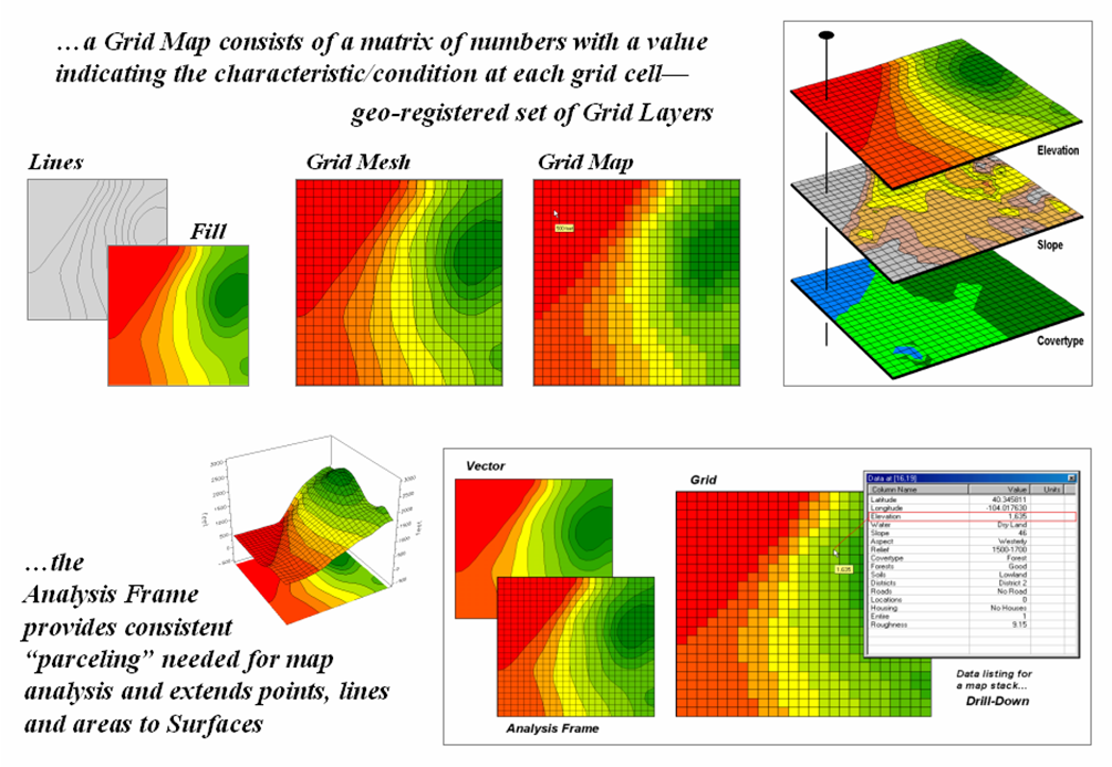
Figure
2. The grid-analysis frame is used to
represent geographic space as a continuum.
Connecting the grid
lines at the center of each grid space forms the 3-D plot in the lower-left
portion of the figure. The lengths of
the lines are a function of the elevation difference between the values stored
at adjacent grid spaces. The result is a
“wireframe” plot that forms the peaks and valleys of the spatial distribution
of the mapped data forming the surface.
The color zones identify contour intervals that are draped on the frame. In addition to providing a format for storing
and displaying map surfaces, the analysis frame provides the consistent
structuring needed for advanced grid-based analysis operations.
Spatial Statistics and Analysis
Grid-based map analysis is
often used in natural resources management and land use planning. However, some of its most innovative
applications have been in disciplines with minimal mapping legacy. The following discussions focus on
geo-business applications to illustrate the Spatial Statistics and Spatial
Analysis operations ingrained in grid-based map analysis.
The two fundamental Spatial
Statistics capabilities of Surface
Modeling and Spatial Data Mining
are described.
Surface Modeling
Surface modeling involves the
translation of discrete point data into a continuous surface that represents the
geographic distribution of data.
Traditional non-spatial statistics involves an analogous process when a
numerical distribution (e.g., standard normal curve) is used to generalize the
central tendency of a data set. The
derived mean (average) and standard deviation reflects the typical response and
provides a measure of how typical it is.
This characterization seeks to explain data variation in terms of the
numerical distribution of measurements without any reference to their spatial
distribution.
In fact, an underlying
assumption in most statistical analyses is that the data is randomly
distributed in space. If the data
exhibits spatial autocorrelation many of the analysis techniques are less
valid.
Spatial statistics, on the
other hand, utilizes geographic patterns in the data to further explain the
variance. There are numerous techniques for characterizing the spatial
distribution inherent in a data set but they can be characterized by three
basic approaches:
-
Point Density mapping that aggregates the number of points within a
specified distance (number per acre),
-
Spatial
Interpolation that weight-averages
measurements within a localized area (e.g., kriging), and
-
Map
Generalization that fits a functional
form to the entire data set (e.g., polynomial surface fitting).
For example, consider Figure
3 showing a point density map derived from customer addresses. The project area is divided into an analysis
frame of 250-foot grid cells (100c x 100r = 10,000 cells). The number of customers for each grid space
is determined street addresses in a desktop mapping system (“spikes” in the 3D
map on the left). A neighborhood summary
operation is used to pass a “roving window” over the project area calculating the
total customers within a half-mile of each map location. The result is a continuous map surface
indicating the relative density of customers—peaks where there is a lot of
customers and valleys where there aren’t many.
In essence, the map surface
quantifies what your eye sees in the spiked map—some areas with lots of
customers and others with very few.
Spatial interpolation also moves a roving window about point data but
utilizes more sophisticated summary techniques, such as Inverse Distance,
Kriging and Minimum Curvature. The
result in either case, are map surfaces that respond to the spatial
distribution in the data.
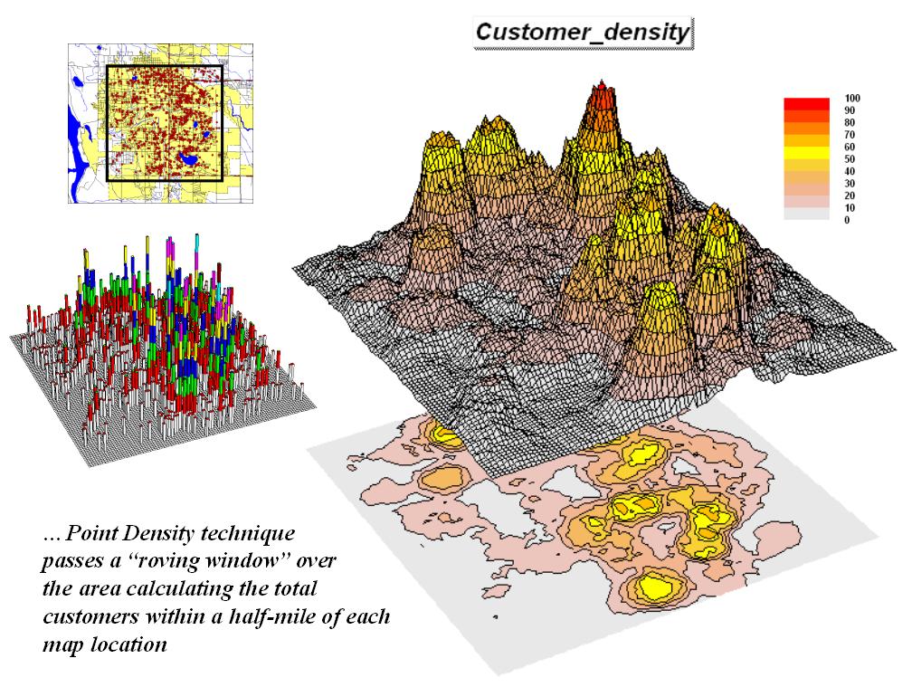
Figure 3. Point
density map aggregating the number of customers within a quarter of a mile.
An underlying assumption of
surface modeling is that that the variable under study forms a gradient in
geographic space (termed “isopleth” data).
The derived surface is an approximation of that gradient. A further assumption is that the data
exhibits spatial autocorrelation—“nearby things are more alike than distant
things.” While some maps containing
discrete objects do not have these qualities, many business decision variables,
such as sales and demographics, express themselves as spatially auto-correlated
gradients. In these instances, surface
modeling is a viable approach to characterizing the geographic distribution of
point-sampled data.
Spatial Data Mining
Spatial data mining seeks to
describe relationships within and among mapped data utilizing techniques such
as coincidence summary, proximal alignment, statistical tests, percent
difference, surface configuration, level-slicing, map similarity, and
clustering in comparing maps and assessing similarities in data patterns.
Another group of spatial data
mining techniques focuses on developing predictive models. For example, the customer density map
described in the previous section might be strongly related to mapped data of
demographics. If that is the case, a
mathematical (or “map-ematical”)
prediction equation can be derived.
Simple linear regression, often used in research, can be applied to a
stack of grid maps—they are just an organized set of numbers awaiting analysis. In essence, the technique goes to a grid
location and notes the density of customers (dependent variable) and the
demographic information, (independent variables) and quantifies the data
pattern. As the process is repeated for
thousands of cells a predictable pattern between the density values and the
demographic values often emerges. If the
relationship is strong, the regression equation can be used to predict a map of
expected customer levels for another city slated for a new office.
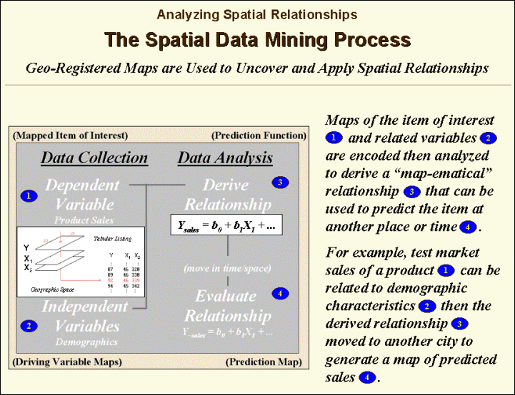
Figure 4.
Spatial data mining can be used to derive predictive models
of the relationships among mapped data.
For example, predictive
modeling was used in the early 1990s to extend a test market project for a
phone company (figure 4). The customer’s
address was used to geo-code sales of a new product that enabled two numbers
with distinctly different rings to be assigned to a single home phone—one for
the kids and one for the parents. Like
pushpins on a map, the pattern of sales throughout the city emerged with some
areas doing very well, while in other areas sales were few and far
between.
The demographic data for
the city was analyzed to calculate a prediction equation between product sales
and census block data. The prediction
equation derived from the test market sales in one city was applied to another
city by evaluating exiting demographics to “solve the equation” for a predicted
sales map. In turn the predicted map was
combined with a wire-exchange map to identify switching facilities that
required upgrading before release of the product in the
A couple of considerations
are important in predictive modeling.
First, the mapped data needs to form spatially auto-correlated gradients
as previously mentioned. Secondly, traditional
multivariate techniques assume that the data values are not categorical or
binary (such as male/female), as the regression technique needs a continuum of
values (such as income levels) to work properly. However, there are other more advanced predictive
techniques (such as CART technology) that can utilize nominal data types.
Spatial data mining
approaches have been used for years in automated classification of remote
sensing data. In these instances,
spectral values are analyzed for a stack of grid layers. Geo-business spatial data mining applications
simply relate grid layers that characterize other information. In addition, geo-business applications focus
more on predictive statistics than descriptive classification.
Cutting-edge research in
spatial data mining is pushing the envelope from descriptive and predictive
statistics to “prescriptive” modeling that seeks to spatially optimize
management action. An example is the
generation of a prescription map in precision agriculture that changes a
fertilization program throughout a field based on the current distribution of
nutrients and yield prediction.
Variable-rate technology actually alters the blend of nutrients
“on-the-fly” as a GPS-equipped spray rig moves across the field. Future decision support systems for business will
likely implement prescriptive modeling based on predictive/descriptive
statistics derived from mapped data.
These systems will generate spatially responsive guidance—“do this over
here but that over there”—that fully incorporates the geographic distribution
inherent in mapped data.
Spatial Analysis
Whereas surface modeling
and spatial data mining respond to “numerical” relationships in mapped data,
spatial analysis is used to investigates the “contextual” relationships. Tools such as slope/aspect, buffers,
effective proximity, optimal path, visual exposure and shape analysis, fall
into this class of spatial operators.
Rather than statistical analysis of mapped data, these techniques
examine geographic patterns, vicinity characteristics and connectivity among
features.
An example of this group of
operations builds on two specific map analysis capabilities—effective proximity
and accumulation surface analysis. The
following discussion focuses on the application of these tools to competition analysis
between two stores.
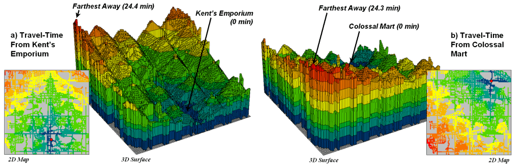
Figure 5. Travel-time surfaces show increasing distance
from a store considering the relative speed along different road types.
The left side of figure 5
shows the travel-time surface from
The result is the estimated
travel-time to every location in the city.
The surface starts at 0 and extends to 24.4 minutes away. Note that it is shaped like a bowl with the
bottom at the store’s location. In the
2D display, travel-time appears as a series of rings—increasing distance
zones. The critical points to
conceptualize are 1) that the surface is analogous to a football stadium
(continually increasing) and 2) that every road location is assigned a distance
value (minutes away).
The right side of figure 5
shows the travel-time surface for another store, Colossal Mart, with its origin
in the northeast portion of the city.
The perspective in both 3D displays is consistent and
Simply subtracting the two
surfaces derives the relative travel-time advantage for the stores (figure
6). Keep in mind that the surfaces
actually contain geo-registered values and a new value (difference) is computed
for each map location. The inset on the
left side of the figure shows a computed Colossal Mart advantage of 6.1 minutes
(22.5 – 16.4= 6.1) for the location in the extreme northeast corner of the
city.
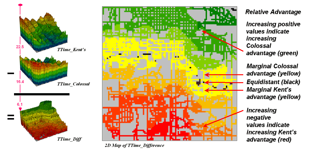
Figure
6. Two travel-time surfaces can be
combined to identify the relative advantage of each store.
Locations that are the same
travel distance from both stores result in zero difference and are displayed as
black. The green tones on the difference
map identify positive values where
 `
`
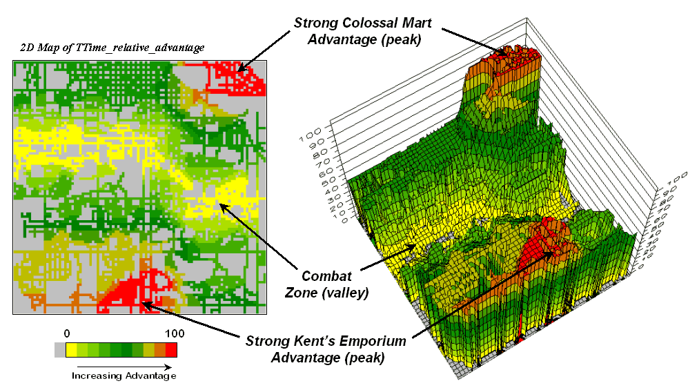
Figure
7. A transformed display of the
difference map shows travel-time advantage as peaks (red) and locations with
minimal advantage as an intervening valley (yellow).
Figure 7 displays the same
information in a bit more intuitive fashion.
The combat zone is shown as a yellow valley dividing the city into two
marketing regions—peaks of strong travel-time advantage. Targeted marketing efforts, such as leaflets,
advertising inserts and telemarketing might best be focused on the combat
zone. The similarity of travel-time to
either store in the combat zone suggests that residents might be more receptive
to store incentives.
At a minimum the travel-time
advantage map enables retailers to visualize the lay of the competitive
landscape. However the information is in
quantitative form and can be readily integrated with other customer data. Knowing the relative travel-time advantage
(or disadvantage) of every street address in a city can be a valuable piece of
the marketing puzzle. Like age, gender,
education, and income, relative travel-time advantage is part of the soup that
determines where one shops.
There are numerous other
map analysis operations in the grid-based “toolbox”—too many to enumerate and
fully discuss in this paper. The
travel-time and competition analysis examples merely illustrate a couple of
geo-business applications capitalizing on the new tools. Motivated readers are encouraged to use the
online links in the References section to extend the discussion.
Conclusion
In many respects map analysis
is as different as it is similar to desktop mapping. While a majority of the extended capabilities
are conceptually intuitive and have been known for decades, their practical
application has been shrouded in complex and expensive software that has kept
map analysis out of most classrooms. The
Instructor’s CD for Map Analysis contains a comprehensive set of educational
materials providing both lecture notes and hands-on exercises in applying this
powerful yet often overlooked side of
References
·
The hardcopy book
and companion CD, Map Analysis: Understanding Spatial Patterns and
Relationships, is designed to support the course and workshop materials in
the Instructor CD for Grid-based Map Analysis.
The CD contains single-seat license for MapCalc Learner and Surfer
software.
(
·
The Beyond Mapping III online book
is a compilation of popular “Beyond Mapping” columns containing twenty-seven
chapters discussing various aspects of grid-based analysis.
(posted
at www.innovativegis.com/basis/MapAnalysis/ )
·
The MapCalc
Learner-Academic software is designed for students and teachers who want
“hands-on” experience with the concepts, procedures and considerations of
grid-based analysis. The single-seat
MapCalc Learner version for students is US$ 21.95; the multi-seat MapCalc Academic
for instructors designed for computer lab use is US$ 495.
(see
www.redhensystems.com,
select Productsà MapCalc)
A
review of MapCalc Learner-Academic software is posted at…
(see
www.innovativegis.com/basis/present/GW01_MCreview/GW_JUN01_mapcalcReview.htm)
________________________
1Joseph K. Berry is a leading consultant and educator in the application of Geographic Information Systems (GIS) technology. He is the Principal of BASIS, consultants and software developers in GIS and the author of the “Beyond Mapping” column for GeoWorld magazine. He has written over two hundred papers on the theory and application of map analysis, and is the author of the popular books Beyond Mapping and Spatial Reasoning. Since 1976, he has presented college courses and professional workshops on GIS to thousands of individuals from a wide variety of disciplines. Dr. Berry conducted basic research and taught courses in GIS for twelve years at Yale University's Graduate School of Forestry and Environmental Studies, and is currently a Special Faculty member at Colorado State University and the W. M. Keck Visiting Scholar in Geography at the University of Denver. He holds a B.S. degree in forestry, an M.B.A. in business management and a Ph.D. emphasizing remote sensing and land use planning.