Infusing Grid-Based Map Analysis Into
Geo-Business Decisions
Joseph K. Berry1
and David Wright2
Berry &
Associates // Spatial Information Systems
2000 South
College Avenue, Suite 300, Fort Collins, Colorado, USA 80525
Phone:
970-215-0825, Email: jberry@innovativegis.com
Abstract
Business applications of
desktop mapping have skyrocketed. The
ability to geo-query databases and visualize the results in a variety of
thematic map forms has developed an appreciation of “where” as well as “what”
in business solutions. However, the
infusion of grid-based map analysis in geo-business has not been as
widespread. While vector-based
approaches are ideal for spatial database management, grid-based analysis
supports mathematical/statistical approaches for quantifying spatial
relationships within and among maps.
This paper describes the similarities and differences between the two
approaches, identifies considerations in their use and presents several
examples of surface modeling, spatial data mining and analysis techniques.
Note: this paper broadly outlines
the major groups of grid-based operators.
Readers are encouraged to use the online links in the References section
to extend the discussions presented in this paper and obtain educational
software for hands-on experience.
Introduction
Vector-based desktop
mapping applications are rapidly becoming part of the modern business
environment. The close link between
these systems and traditional spreadsheet and database management programs has
fueled the adoption. In many ways, a
“database is just picture waiting to happen.”
The direct link between the attributes described in a database record
and its spatial characterization is conceptually easy. Geo-query by clicking on a map to pop-up the
attribute record or searching a database then plotting the selected records is
an extremely useful extension of traditional database technology. Couple decreasing desktop mapping system
costs and complexity with increasing data availability and Internet access makes
the adoption of spatial database technology a “no-brainer.” Maps in their traditional form of point,
lines and polygons identifying discrete spatial object align with manual
mapping concepts and experiences learned as early as girl and boy scouts.
Grid-based maps, on
the other hand, represent a different paradigm of geographic space. Whereas traditional vector maps emphasize
“precise placement of physical features,” grid maps seek to “statistically characterize
continuous space in both real and cognitive terms.” The tools for mapping of database attributes are extended to
analysis of spatial relationships. This
paper describes some of the basic concepts, considerations and procedures in
grid-based data handling and analysis operations as they apply to geo-business
applications. Three fundamental
capabilities are discussed—surface modeling, spatial data mining and map
analysis.
Surface Modeling
Surface modeling involves
the translation of discrete point data into a continuous surface that
represents the geographic distribution of data. Traditional non-spatial statistics involves an analogous process
when a numerical distribution (e.g., standard normal curve) is used to
generalize the central tendency of a data set.
The derived mean (average) and standard deviation reflects the typical
response and provides a measure of how typical it is. This characterization seeks to explain data variation in terms of
the numerical distribution of measurements without any reference to their
spatial distribution.
In fact, an
underlying assumption in most statistical analyses is that the data is randomly
distributed in space. If the data
exhibits spatial autocorrelation many of the analysis techniques are less
valid.
Spatial statistics,
on the other hand, utilizes geographic patterns in the data to further explain
the variance. There are numerous techniques for characterizing the spatial
distribution inherent in a data set but they can be characterized by three
basic approaches:
·
Point
Density mapping that
aggregates the number of points within a specified distance (number per acre),
·
Spatial
Interpolation that
weight-averages measurements within a localized area (e.g., kriging), and
·
Map Generalization that fits a functional form to the entire
data set (e.g., polynomial surface fitting).
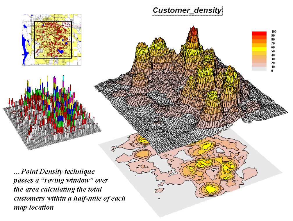 Figure 1-1. Point density
map aggregating the number of customers within a quarter of a mile.
Figure 1-1. Point density
map aggregating the number of customers within a quarter of a mile.
For example, consider
Figure 1-1 showing a point density map derived from customer addresses. The project area is divided into an analysis
frame of 250-foot grid cells (100c x 100r = 10,000 cells). The number of customers for each grid space
is determined street addresses in a desktop mapping system (“spikes” in the 3D
map on the left). A neighborhood
summary operation is used to pass a “roving window” over the project area
calculating the total customers within a half-mile of each map location. The result is a continuous map surface
indicating the relative density of customers—peaks where there is a lot of
customers and valleys where there aren’t many.
In essence, the map
surface quantifies what your eye sees in the spiked map—some areas with lots of
customers and others with very few. Spatial
interpolation also moves a roving window about point data but utilizes more sophisticated
summary techniques, such as Inverse Distance, Kriging and Minimum Curvature. The result in either case, are map surfaces
that respond to the spatial distribution in the data.
An underlying
assumption of surface modeling is that that the variable under study forms a
gradient in geographic space (termed “isopleth” data). The derived surface is an approximation of
that gradient. A further assumption is
that the data exhibits spatial autocorrelation—“nearby things are more alike
than distant things.” While some maps containing
discrete objects do not have these qualities, many business decision variables,
such as sales and demographics, express themselves as spatially auto-correlated
gradients. In these instances, surface
modeling is a viable approach to characterizing the geographic distribution of
point-sampled data.
Spatial Data Mining
Spatial data mining seeks to uncover relationships within and among mapped data. A companion paper presented at this conference, entitled “Quantitative Methods for Analyzing Map Similarity and Zoning” describes some of the techniques—coincidence summary, proximal alignment, statistical tests, percent difference, surface configuration, level-slicing, map similarity, and clustering—used in comparing maps and assessing similarities in data patterns.
Another group of spatial data mining techniques focuses on developing predictive models. For example, the customer density map described in the previous section might be strongly related to mapped data of demographics. If that is the case, a mathematical (or “map-ematical”) prediction equation can be derived. Simple linear regression, often used in research, can be applied to a stack of grid maps—they are just an organized set of numbers awaiting analysis. In essence, the technique goes to a grid location and notes the density of customers (dependent variable) and the demographic information, (independent variables) and quantifies the data pattern. As the process is repeated for 10,000 cells a predictable pattern between the density values and the demographic values often emerges. If the relationship is strong, the regression equation can be used to predict a map of expected customer levels for another city slated for a new office.
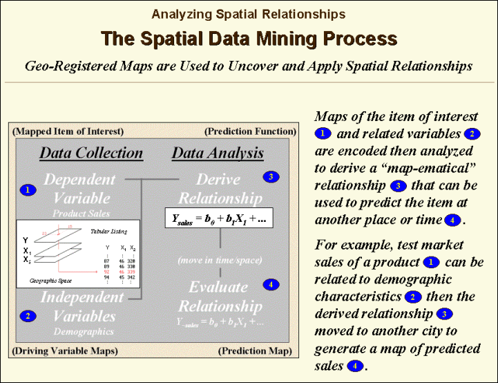 Figure 1-2. Spatial
data mining can be used to derived predictive models of the relationships among
mapped data.
Figure 1-2. Spatial
data mining can be used to derived predictive models of the relationships among
mapped data.
For example, an early use
of predictive modeling was in extending a test market project for a phone
company. The customer’s address was
used to geo-code sales of a new product that enabled two numbers with
distinctly different rings to be assigned to a single phone—one for the kids
and one for the parents. Like pushpins
on a map, the pattern of sales throughout the city emerged with some areas
doing very well, while in other areas sales were few and far between.
The demographic data for
the city was analyzed to calculate a prediction equation between product sales
and census block data. The prediction
equation derived from the test market sales in one city was applied to another
city by evaluating exiting demographics to “solve the equation” for a predicted
sales map. In turn the predicted map
was combined with a wire-exchange map to identify switching facilities that
required upgrading before release of the product in the new city.
A couple of considerations
are important in predictive modeling. First,
the mapped data needs to form spatially auto-correlated gradients as previously
mentioned. Secondly, traditional
multivariate techniques assume that the data values are not categorical or
binary (such as male/female), as the regression technique needs a continuum of
values (such as income levels) to work properly. However, there are other more advanced predictive techniques (such
as CART technology) that can utilize nominal data types.
Spatial data mining approaches
have been used for years in automated classification of remote sensing
data. In these instances, spectral values
are analyzed for a stack of grid layers.
Geo-business spatial data mining applications simply relate grid layers
that characterize other information. In
addition, geo-business applications focus more on predictive statistics than
descriptive classification.
Cutting-edge research in
spatial data mining is pushing the envelop from descriptive and predictive
statistics to prescriptive modeling that seeks to spatially optimize management
action. An example is the generation of
a prescription map in precision agriculture that changes a fertilization
program throughout a field based on the current distribution of nutrients and
yield prediction. Variable-rate
technology actually alters the blend of nutrients “on-the-fly” as a GPS-equipped
spray rig moves across the field. Future
decision support systems for business will likely implement prescriptive
modeling based on predictive/descriptive statistics derived from mapped
data. These systems will generate spatially
responsive guidance—“do this over here but that over there”—that fully
incorporates the geographic distribution inherent in mapped data.
Map Analysis
Whereas spatial data mining
responds to “numerical” relationships in mapped data, map analysis investigates
the “contextual” relationships. Tools
such as slope/aspect, buffers, effective proximity, optimal path, visual
exposure and shape analysis, fall into this class of spatial operators. Rather than statistical analysis of mapped
data, these techniques examine geographic patterns, vicinity characteristics
and connectivity among features.
A example of this group of operations
builds on two specific map analysis capabilities—effective proximity and accumulation
surface analysis. The following
discussion focuses on the application of these tools to competition analysis
between two stores.
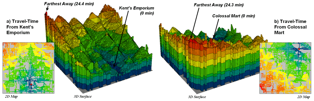 Figure 1-3. Travel-time surfaces show increasing
distance from a store considering the relative speed along different road
types.
Figure 1-3. Travel-time surfaces show increasing
distance from a store considering the relative speed along different road
types.
The left side of figure 1-3 shows the travel-time surface from Kent’s Emporium. It is calculated by starting at the store then moving out along the road network like waves propagating through a canal system. As the wave front moves, it adds the time to cross each successive road segment to the accumulated time up to that point.
The result is the estimated travel-time to every location in the city. The surface starts at 0 and extends to 24.4 minutes away. Note that it is shaped like a bowl with the bottom at the store’s location. In the 2D display, travel-time appears as a series of rings—increasing distance zones. The critical points to conceptualize are 1) that the surface is analogous to a football stadium (continually increasing) and 2) that every road location is assigned a distance value (minutes away).
The right side of figure 1-3 shows the travel-time surface for another store, Colossal Mart, with its origin in the northeast portion of the city. The perspective in both 3D displays is consistent and Kent’s surface appears to “grow” away from you while Colossal’s surface seems to grow toward you.
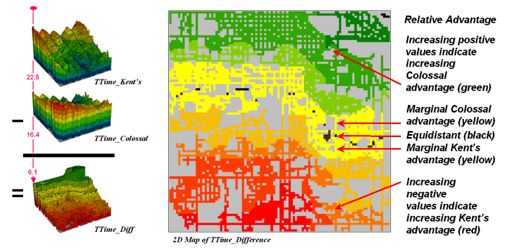 Figure
1-4. Two travel-time surfaces can be
combined to identify the relative advantage of each store.
Figure
1-4. Two travel-time surfaces can be
combined to identify the relative advantage of each store.
Simply subtracting the two surfaces derives the relative travel-time advantage for the stores (figure 1-4). Keep in mind that the surfaces actually contain geo-registered values and a new value (difference) is computed for each map location. The inset on the left side of the figure shows a computed Colossal Mart advantage of 6.1 minutes (22.5 – 16.4= 6.1) for the location in the extreme northeast corner of the city.
Locations that are the same travel distance from both stores result in zero difference and are displayed as black. The green tones on the difference map identify positive values where Kent’s travel-time is larger than its competitor’s—advantage to Colossal Mart. Negative values (red tones) indicate the opposite—advantage to Kent’s Emporium. The yellow tone indicates the “combat zone” where potential customers are about the same distance from either store—advantage to no one.
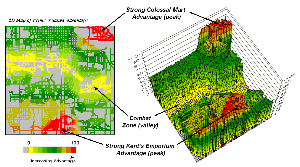 Figure
1-5. A transformed display of the
difference map shows travel-time advantage as peaks (red) and locations with
minimal advantage as an intervening valley (yellow).
Figure
1-5. A transformed display of the
difference map shows travel-time advantage as peaks (red) and locations with
minimal advantage as an intervening valley (yellow).
Figure 1-5 displays the same information in a bit more intuitive fashion. The combat zone is shown as a yellow valley dividing the city into two marketing regions—peaks of strong travel-time advantage. Targeted marketing efforts, such as leaflets, advertising inserts and telemarketing might best be focused on the combat zone. Indifference towards travel-time means that the combat zone residents might be more receptive to store incentives.
At a minimum the travel-time advantage map enables retailers to visualize the lay of the competitive landscape. However the information is in quantitative form and can be readily integrated with other customer data. Knowing the relative travel-time advantage (or disadvantage) of every street address in a city can be a valuable piece of the marketing puzzle. Like age, gender, education, and income, relative travel-time advantage is part of the soup that determines where one shops.
There are numerous other map
analysis operations in the grid-based “toolbox”—too many to enumerate and fully
discuss in this paper. The travel-time
and competition analysis examples merely illustrate a couple of geo-business
applications capitalizing on the new tools.
Motivated readers are encouraged to use the online links in the
References section to extend the discussion.
Conclusion
Vector-based systems for
mapping and spatial database management are gaining a solid foothold in
business. Their thematic mapping and
geo-query capabilities align with and extend traditional data processing
approaches. Grid-based systems, on the
other hand, involve new data structures, storage/retrieval procedures and
entirely new analysis paradigms. Its surface
modeling, spatial data mining and map analysis approaches better align with
statistics and mathematics—an important but often secondary side of information
systems technology. These procedures, however, support new ways
of conceptualizing, expressing and modeling business systems. The explicit consideration of numerical and
contextual relationships within and among mapped data can provide new insight and
solution approaches to complex problems.
Consideration of “where,” as well as “what,” is a natural extension to
business decision-making. The computer
systems, data and access for infusing grid-based analysis into geo-business decisions
are at hand—what remains is infusing the techniques into the business mindset.
References
The online book, Map
Analysis (available at www.innovativegis.com/basis/MapAnalysis/Default.html)
is a compilation of popular “Beyond Mapping”
columns published in GEOWorld magazine from 1996 through 2001. It contains seventeen chapters discussing various
aspects of grid-based analysis including surface modeling (Topics 2, 3 and 8),
spatial data mining (Topics 7,10 and 16) and map analysis (Topics 5,6,14 and
17). Motivated readers are encouraged
to review these sections to extend the discussions in this paper.
The MapCalc Learner-Academic system (see www.redhensystems.com, select Productsà MapCalc) is designed for students and teachers who want “hands-on” experience with the concepts, procedures and considerations of grid-based analysis. A companion paper presented at this conference, entitled “Infusing Grid-Based Map Analysis Into Introductory GIS Courses” describes the educational software and materials for classroom and self-learning. The MapCalc Learner version for students is US$ 21.95; MapCalc Academic for instructors is US$ 495 plus shipping and handling.
_______________________
1Joseph
K. Berry is a leading consultant and educator in the application of Geographic
Information Systems (GIS) technology.
He is the president of BASIS, consultants and software developers in GIS
and the author of the “Beyond Mapping” column for GEOWorld magazine. He has written over two hundred papers on
the theory and application of map analysis, and is the author of the popular
books Beyond Mapping and Spatial Reasoning. Since 1976, he has presented workshops on
GIS to thousands of individuals from a wide variety of disciplines. Dr. Berry conducted basic research and
taught courses in GIS for twelve years at Yale University's Graduate School of
Forestry and Environmental Studies, and is currently a Special Faculty member
at Colorado State University and the W. M. Keck Visiting Scholar in Geography
at the University of Denver. He holds a
B.S. degree in forestry, an M.B.A. in business management and a Ph.D. emphasizing
remote sensing and land use planning.
2 David Wright is a Research and Development Manager at
Red Hen Systems, Fort Collins, Colorado, Email dkwright@redhensystems.com.