Bridging GIS and Map Analysis:
Identifying and Utilizing Spatial
relationships
Joseph K. Berry
Keck Scholar in Geosciences,
Principal, Berry & Associates // Spatial
Information Systems (BASIS)
ABSTRACT
Most human
endeavors are inherently spatial. The
world we live in surrounds us with opportunities and challenges that are
spatially dependent on “Where is What”
tempered by “Why and So What” within
cognitive contexts. In just three decades
GIS technology has revolutionized our perspective on what constitutes a map and
the information it can project. The
underlying data are complex, as two descriptors are required— precise location,
as well as a clear description. Manually
drafted maps emphasized accurate location of physical features. Today, maps have evolved from guides of
physical space into management tools for exploring spatial relationships and
perceptions. The journey from the map
room to the conference room has transformed maps from static wall hangings into
interactive mapped data that address complex spatial issues. It also has sparked an entirely new
analytical tool set that provides needed insight for effective decision-making. This new perspective marks a turning point in
the use of maps— from one emphasizing physical descriptions of geographic
space, to one of interpreting mapped data and successfully communicating
spatially based decision factors. This
paper investigates the context, conditions and forces forming the bridge
from maps to mapped data, spatial analysis and beyond.
INTRODUCTION
Map analysis tools might at first seem uncomfortable,
but they are simply extensions of traditional analysis procedures brought on by
the digital nature of modern maps. Since
maps are “number first, pictures later,” a map-ematical framework can be
can be used to organize the analytical operations. Like basic math, this approach uses
sequential processing of mathematical operations to perform a wide variety of
complex map analyses. By controlling the
order which the operations are executed, and using a common database to store
the intermediate results, a mathematical-like processing structure is
developed.
This “map algebra” was first suggested in the late
1970s in a doctoral dissertation by Dana Tomlin while at
In grid-based map analysis, the spatial coincidence and juxtapositioning of
values among and within maps create new analytical operations, such as
coincidence, proximity, visual exposure and optimal routes. These operators are accessed through general
purpose map analysis software available in many GIS systems, such as MapCalc,
GRASS, ERDAS or the Spatial Analyst extension to ArcGIS. While the specific command syntax and
mechanics differs among software brands, the basic analytical capabilities and
spatial reasoning skills used in map analysis form a common foundation.
FUNDAMENTAL CONDITIONS FOR MAP ANALYSIS
There are two fundamental conditions required by any
map analysis package—a consistent data structure and an iterative
processing environment. Topic 18 in
the online book Map Analysis (
The second condition of map analysis provides an
iterative processing environment by logically sequencing map analysis
operations and serves as the focus of this paper. This involves:
¾ retrieval of one or more map layers from the database,
¾ processing that data as specified by the user,
¾ creation of a new map containing the processing results, and
¾ storage of the new map for subsequent processing.
Each new map derived as processing continues aligns
with the analysis frame so it is automatically geo-registered to the other maps
in the database. The values comprising
the derived maps are a function of the processing specified for the “input
maps.”
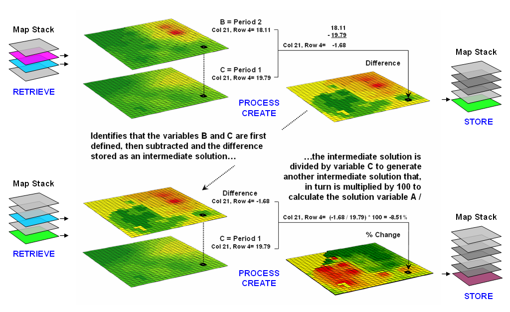
Figure 1. An iterative processing environment,
analogous to basic math, is used to derive new map variables.
This cyclical processing provides an extremely flexible
structure similar to “evaluating nested parentheticals” in traditional
math. Within this structure, one first
defines the values for each variable and then solves the equation by performing
the mathematical operations on those numbers in the order prescribed by the
equation. For example, the equation for
calculating percent change in your investment portfolio—
%Change
= A = ( B - C ) / C ) * 100
=
( 100,000 – 90,000 ) / 90,000 ) * 100 …define
variables
=
( 10,000 ) / 90,000 ) *100 …intermediate
solution #1
=
( .111 ) * 100 …intermediate
solution #2
=
11.1 % …final
solution
—identifies that the variables B and C are first
defined, then subtracted and the difference stored as an intermediate
solution. The intermediate solution is
divided by variable C to generate another intermediate solution that, in turn
is multiplied by 100 to calculate the solution variable A.
This same basic mathematical structure provides the
framework for computer-assisted map analysis.
The only difference is that the variables are represented by mapped data
composed of thousands of values organized into a grid. Figure 1 shows a similar solution for
calculating percent change in animal activity based on mapped data.
The processing steps shown in the figure are identical
to the traditional solution except the calculations are performed for each grid
cell in the study area and the result is a map that identifies the percent
change at each map location. Map analysis
identifies what kind of change (termed the thematic attribute) occurred where
(termed the spatial attribute). The
characterization of what and where provides information needed
for further GIS modeling, such as determining if areas of large increases in
animal activity are correlated with particular cover types or near areas of low
human activity.
FUNDAMENTAL MAP ANALYSIS OPERATIONS
Within this iterative processing structure, four
fundamental classes of map analysis operations can be identified. These include:
¾ Reclassifying
Maps that involve
the reassignment of the values of an existing map as a function of its initial
value, position, size, shape or contiguity of the spatial configuration
associated with each map category.
¾ Overlaying
Maps that result in the creation of
a new map where the value assigned to each location is computed as a function
of the independent values associated with that location on two or more maps.
¾ Measuring
Distance and Connectivity that
involve the creation of a new map expressing the distance and route between
locations as straight-line length (simple proximity) or as a function of
absolute or relative barriers (effective proximity).
¾ Characterizing
and Summarizing Neighborhoods
that result in the creation of a new map based on the consideration of values
within the general vicinity of target locations.
Reclassification operations merely repackage existing
information on a single map without creating new spatial patterns. Overlay operations, on the other hand,
involve two or more maps and result in the creation of new spatial
patterns. Distance and connectivity
operations are more advanced techniques that generate entirely new information
by characterizing the relative positioning of map features. Neighborhood operations summarize the conditions
occurring in the general vicinity of a location. The online book, Map Analysis (
The reclassifying and overlaying operations based on point
processing are the backbone of current GIS applications, allowing rapid
updating and examination of mapped data.
However, other than the significant advantage of speed and ability to
handle tremendous volumes of data, these capabilities are similar to those of
manual map processing. Map-wide
overlays, distance and neighborhood operations, on the other hand, identify
more advanced analytic capabilities and most often do not have paper-map legacy
procedures.
The mathematical structure and classification scheme
of Reclassify, Overlay, Distance and Neighbors form a conceptual framework that
is easily adapted to modeling spatial relationships in both physical and
abstract systems. A major advantage is
flexibility. For example, a model for
siting a new highway could be developed as a series of processing steps. The analysis likely would consider economic
and social concerns (e.g., proximity to high housing density, visual exposure
to houses), as well as purely engineering ones (e.g., steep slopes, water
bodies). The combined expression of both
physical and non-physical concerns within a quantified spatial context is a
major benefit.
The ability to simulate various scenarios (e.g.,
steepness is twice as important as visual exposure and proximity to housing is
four times more important than all other considerations) provides an
opportunity to fully integrate spatial information into the decision-making
process. By noting how often and where
the proposed route changes as successive runs are made under varying
assumptions, information on the unique sensitivity to siting a highway in a
particular locale is described.
In addition to flexibility, there are several other
advantages in developing a generalized analytical structure for map
analysis. The systematic rigor of a
mathematical approach forces both theorist and user to carefully consider the
nature of the data being processed. Also
it provides a comprehensive format for learning that is independent of specific
disciplines or applications. Furthermore
the flowchart of processing succinctly describes the components and weightings
capsulated in an analysis.
This communication enables decision-makers to more
fully understand the analytic process and actually interact with weightings,
incomplete considerations and/or erroneous assumptions. These comments, in most cases, can be easily
incorporated and new results generated in a timely manner. From a decision-maker’s point of view,
traditional manual techniques for analyzing maps are a distinct and separate
task from the decision itself. They
require considerable time to perform and many of the considerations are
subjective in their evaluation.
In the old environment, decision-makers attempt to
interpret results, bounded by vague assumptions and system expressions of the
technician. Computer-assisted map
analysis, on the other hand, engages decision-makers in the analytic
process. In a sense, it both documents
the thought process and encourages interaction—sort of like a “spatial
spreadsheet.”
MAPPING VERSUS
ANALYSIS
Vector-based desktop mapping
is rapidly becoming part of the modern business environment. The close link between these systems and
traditional spreadsheet and database management programs has fueled the
adoption. In many ways, “a database
is just picture waiting to happen.”
The direct link between attributes described in a database record and
their spatial characterization is conceptually easy. Geo-query by clicking on a map to pop-up the
attribute record or searching a database then plotting the selected records is
an extremely useful extension of contemporary procedures. Increasing data availability and Internet
access coupled with decreasing desktop mapping system costs and complexity make
adoption of spatial database technology a practical reality.
Maps in their traditional
form of point, lines and polygons identifying discrete spatial objects align
with manual mapping concepts and experiences learned as early as girl and boy
scouts. Grid-based maps, on the other
hand, represent a different paradigm of geographic space. Whereas traditional vector maps emphasize “precise
placement of physical features,” grid maps seek to “statistically
characterize continuous space in both real and cognitive terms.” The tools for mapping of database attributes
are extended to analysis of spatial relationships. This paper focuses the basic concepts,
considerations and procedures in map analysis operations as they apply to many
disciplines. Three broad capabilities
are discussed—1) surface modeling, 2) spatial data mining and 3) spatial
analysis.
SURFACE MODELING
Surface modeling involves the translation of discrete point data into a continuous
surface that represents the geographic distribution of that data. Traditional non-spatial statistics involves
an analogous process when a numerical distribution (e.g., standard normal
curve) is used to generalize the central tendency of a data set. The derived mean (average) and standard
deviation reflects the typical response and provides a measure of how typical
it is. This characterization seeks to
explain data variation in terms of the numerical distribution of measurements
without any reference to the data’s spatial distribution.
In fact, an underlying
assumption in most traditional statistical analyses is that the data is
randomly distributed in space. If the
data exhibits spatial autocorrelation, many of the analysis techniques are less
valid. Spatial statistics, on the other
hand, utilizes geographic patterns in the data to further explain the
variance. There are numerous techniques
for characterizing the spatial distribution inherent in a data set but they can
be characterized by three basic approaches:
¾
Point Density mapping that aggregates the number of points within a specified
distance (number per acre),
¾
Spatial Interpolation that weight-averages measurements within a localized
area (e.g., kriging), and
¾
Map Generalization that fits a functional form to the entire data set
(e.g., polynomial surface fitting).
For example, consider figure
2 showing a point density map derived from customer addresses. The project area is divided into an analysis
frame of 250-foot grid cells (100c x 100r = 10,000 cells). The number of customers for each grid space
is determined by street addresses in a desktop mapping system (“spikes” in the
3D map on the left).
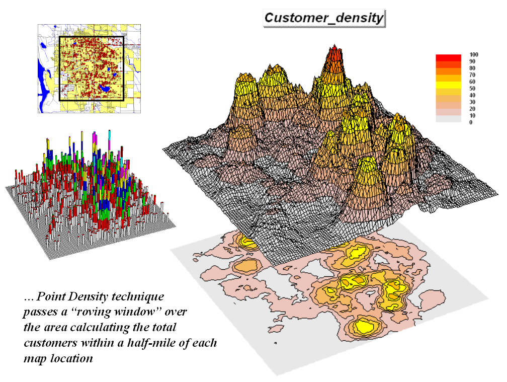
Figure 2. Point
density map aggregating the number of customers within a specified distance.
A neighborhood summary
operation is used to pass a “roving window” over the project area calculating
the total customers within a half-mile of each map location. The result is a continuous map surface
indicating the relative density of customers—peaks where there is a lot of
nearby customers and valleys where there aren’t many. In essence, the map surface quantifies what
your eye sees in the spiked map—some areas with lots of customers and others
with very few.
SPATIAL DATA
MINING
Spatial data mining seeks to uncover relationships within and among
mapped data. Some of the techniques
include coincidence summary, proximal alignment, statistical tests, percent
difference, surface configuration, level-slicing, map similarity, and clustering
that are used in comparing maps and assessing similarities in data
patterns.
Another group of spatial
data mining techniques focuses on developing predictive models. For example, an early use of predictive
modeling was in extending a test market project for a phone company (figure 3). Customers’ address were used to “geo-code”
map coordinates for sales of a new product enabling distinctly different rings
to be assigned to a single phone—one for the kids and one for the parents. Like pushpins on a map, the pattern of sales
throughout test market emerged with some areas doing very well, while in other
areas sales were few and far between.
The demographic data for
the city was analyzed to calculate a prediction equation between product sales
(dependent variable) and census block data (independent variables). The regression equation that was developed is
similar to one derived using non-spatial statistics using a discrete set of
samples. However in the spatial
statistics solution entire map surfaces are considered that account for the spatial
autocorrelation within each map variable.
In addition, the solution is based on thousands of spatially dependent
cases instead of just a few spatially independent samples.
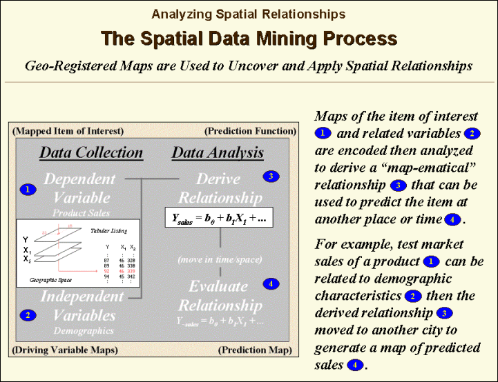
Figure 3.
Spatial data mining can be used to derive predictive models of the
relationships among mapped data.
The prediction equation
derived from the test market sales was then applied to another city by
evaluating existing demographics to “solve the equation” for a predicted sales
map. In turn, the predicted map was
combined with a wire-exchange map to identify switching facilities that would
require upgrading before release of the product in the
The variables used in the
analysis consider geographic space as a continuum of demographic
characteristics and the resultant map as a continuum characterizing the spatial
propensity to purchase a product.
Similar analyses can relate crop yield to soil nutrient levels throughout
a field or animal activity to habitat conditions. The spatial data mining process is
independent of application characteristics and is valid for mapped data that
form continuous distributions in both numerical and geographical space. New statistical techniques, such as CART
technology, that can utilize nominal and ordinal data promise to revolutionize
geoscience, as much as they are revolutionizing traditional statistics.
SPATIAL ANALYSIS
Whereas spatial data mining
responds to “numerical” relationships in mapped data, spatial analysis investigates the “contextual”
relationships. Tools such as
slope/aspect, buffers, effective proximity, optimal path, visual exposure and
shape analysis, fall into this class of spatial operators. Rather than statistical analysis of mapped
data, these techniques examine geographic patterns, vicinity characteristics
and connectivity among features.
The example shown in
figures 4 and 5 builds on two specific map analysis capabilities—effective
proximity and accumulation surface analysis. The following discussion focuses on the
application of these tools to competition analysis between two stores.
The top-left side of figure 4
shows the travel-time surface from
The result is the estimated
travel-time from
The inset below
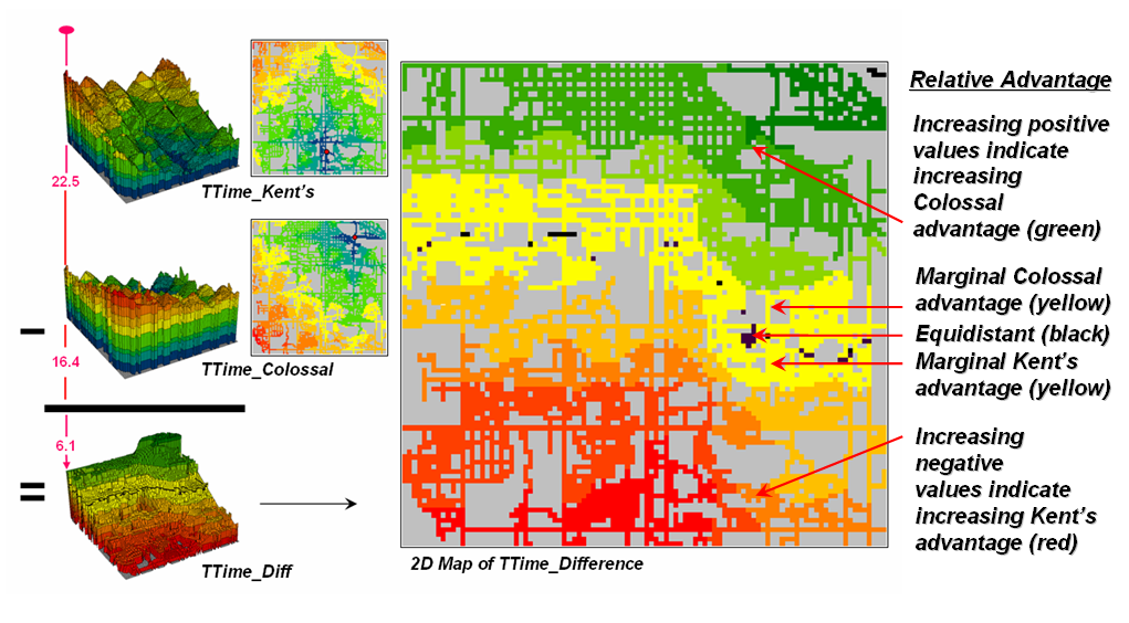
Figure 4. Two
travel-time surfaces can be combined to identify the relative advantage of each
store.
Simply subtracting the two surfaces
derives the relative travel-time advantage for the stores (right-side figure
4). Keep in mind that the surfaces
actually contain geo-registered values and a new value (difference) is computed
for each map location. The inset on the
left side of the figure shows a computed Colossal Mart advantage of 6.1 minutes
(22.5 – 16.4= 6.1) for the indicated location in the extreme northeast corner
of the city.
Locations that are the same
travel distance from both stores result in zero difference and are displayed as
black. The green tones on the difference
map identify positive values where
Figure 5 displays the same
information as a 3D surface. The combat
zone is shown as a yellow valley dividing the city into two marketing
regions—peaks of strong travel-time advantage.
Targeted marketing efforts, such as leaflets, advertising inserts and
telemarketing might best be focused on the combat zone.
At a minimum the travel-time
advantage map enables retailers to visualize the lay of the competitive
landscape. However the information is in
quantitative form and can be readily integrated with other customer data. Knowing the relative travel-time advantage
(or disadvantage) of every street address in a city can be a valuable piece of
the marketing puzzle. Like age, gender,
education, and income, relative travel-time advantage is part of the soup that
determines where one shops.
There are numerous other map
analysis operations in the grid-based “toolbox.” The examples of customer density surface,
sales prediction map and travel-time/competition analysis were used to
illustrate a few of geo-business applications capitalizing on the new
tools. Keep in mind that the tools are
generic and can be applied to a wide variety of spatial problems within most
disciplines. Like traditional
mathematics, the tools are not application specific. They arise from the digital nature of modern
maps to form a generalized map-ematics
that catapults GIS technology beyond mapping and geo-query.
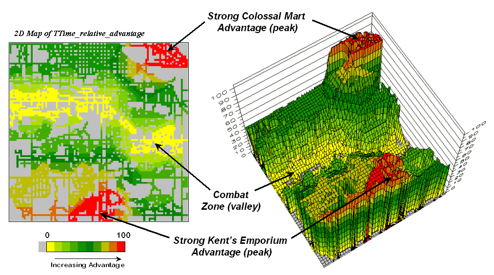
Figure 5. A
transformed display of the difference map shows travel-time advantage as peaks
(red) and locations with minimal advantage as an intervening valley (yellow).
Early information systems
relied on physical storage of data and manual processing. With the advent of the computer, most of
these data and procedures have been automated during the past three
decades. Commensurate with the digital
map, geoscience and resource information processing increasingly has become
more quantitative. Systems analysis techniques developed links between
descriptive data to the mix of management actions that maximize a set of
objectives. This mathematical approach
to geoscience investigation has been both stimulated and facilitated by modern
information systems technology. The
digital nature of mapped data in these systems provides a wealth of new
analysis operations and an unprecedented ability to model complex spatial issues. The full impact of the new data form and
analytical capabilities is yet to be realized.
CONCLUSION
It is certain, however, that
tomorrow's GIS will build on the cognitive basis, as well as the spatial
databases and analytical operations of the technology. This contemporary view pushes GIS beyond simply
mapping and spatial database management to map analysis and spatial reasoning that
focuses on the solution and communication of complex geographic phenomena and
decision contexts. In a sense, the bridge
between GIS and map analysis is formed by the map-ematical structure and fundamental processing operations contained
in grid-based analytical packages. The
bridge takes us to a better understanding of spatial relationships and their
application in solving environmental, economic and social concerns facing an
increasingly complex world.
REFERENCES
Haklay, M.
(2004), Map Calculus in GIS: a proposal and
demonstration. International Journal of Geographical Information
Science, 18 (2):107-125.