DELPHI PROCESS

Applying Delphi in Calibrating GIS Model Criteria

The following extends the brief description in the Beyond Mapping column on “Calibrating and Weighting GIS Model Criteria” by Joseph K. Berry appearing in GeoWorld, September, 2003. The columns in this series are posted at— http://www.innovativegis.com/basis/MapAnalysis/Default.html, select Topic 19, Routing and Optimal Paths.

A companion discussion on applying the Analytical Hierarchy process (AHP) for “weighting GIS model criteria” is posted at— http://www.innovativegis.com/basis/bm/Beyond.htm#BM_supplements.

What is Delphi?

The Delphi Process provides a structured method for developing consensus in areas that are hard to quantify or difficult to predict. It was originally developed in the 1950s by Rand Corporation for forecasting future scenarios but since has been used as a generic strategy for group-based decisions in a variety of fields. The essence of Delphi is structuring of the group communication process aimed at producing detailed critical examination and discussion (Gazing Into the Oracle: The Delphi Method and Its Application to Social Policy and Public Health, by Murray Turoff and Starr Roxanne Hiltz, Kingsley Publishers, London).

What kind of information is gained?

Delphi has been successfully used in a wide variety of applications from military strategy to medical practice, business management methods, sales forecasting and new product development. The procedure is designed to reduce bias and undue influence in group discussion through an ordered and iterative process. It can be used to calibrate the decision elements (map layers) for GIS-based Suitability and Routing models.

What is involved in the process?

The Delphi Process involves anonymity, iteration with controlled feedback (both qualitative and quantitative) and documentation of group interaction. It includes a series of “rounds” that solicit group responses to a set of questions— the answers are tabulated, and the results are used to form the basis for the next round. Through several iterations, this process synthesizes the responses, most often resulting in consensus that reflects the participants' combined intuition and expert knowledge.

Who should be involved?

In the routing of an electric transmission line described in the Beyond Mapping series (see above reference), “Discipline Experts” identify model criteria and conceptual structuring of the problem. “GIS Experts” provide input on data availability, analysis techniques required and technical structuring of the model.

How are the decision elements identified and calibrated?

Two levels of interactive group discussion are involved in developing a GIS model. At the first level, decision elements (map layers) that “drive” the problem are identified and used to structure the model. At the second level, the decision elements are calibrated to reflect the appropriate interpretation of the criteria. Delphi can be useful at both levels and is particularly effective in facilitating communication among GIS and discipline experts.

(Click image to enlarge) In the transmission line routing example, the decision elements are Housing Density, Proximity to Roads, Proximity to Sensitive Areas, and Visual Exposure to Houses (Level 1 discussion). These map layers are derived from base maps of Housing, Roads, Sensitive Areas and Elevation using the MapCalc commands Scan, Spread, and Radiate to create the intermediate “derived” maps.

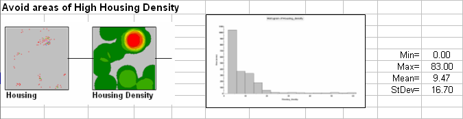
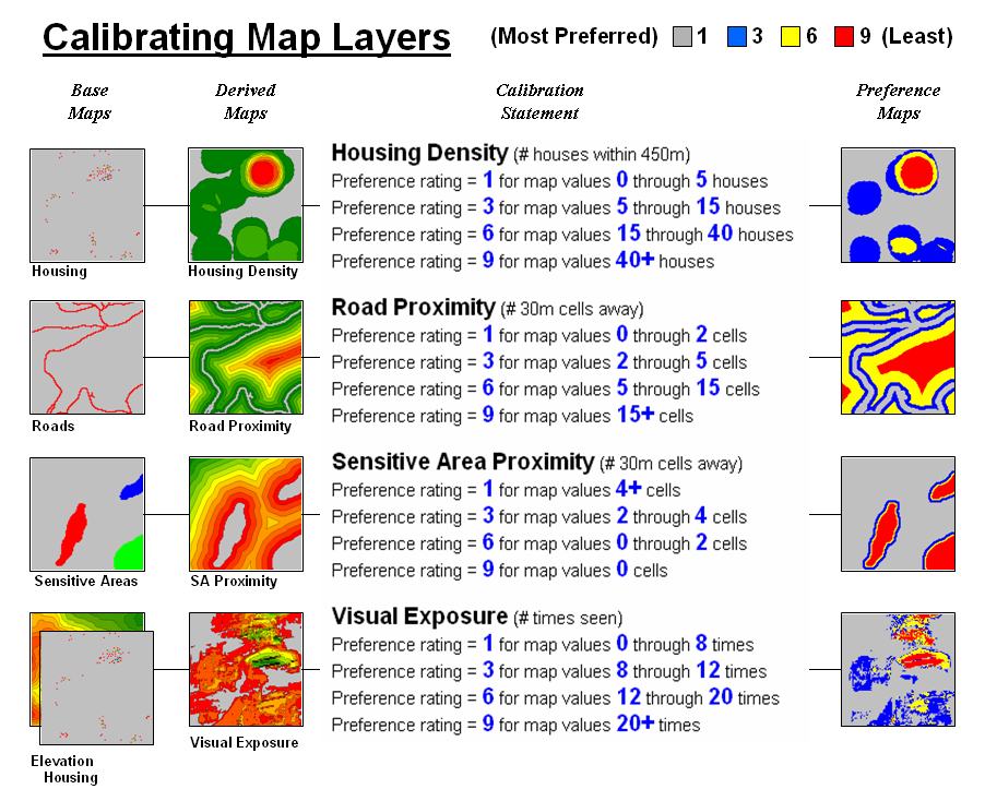
The calibration of the derived maps (Level 2 discussion) reflect the model’s objectives and include avoiding locations that 1) have high Visual Exposure (VE= V_Exposure_rating), 2) are close to Sensitive Areas (SA= SA_Proximity_rating), 3) are close to Roads (R= R_Proximity_rating) and 4) have high Housing Density (HD= H_Density_rating). The MapCalc command Renumber is used to reclassify the derived maps (set the ratings).

The following discussion illustrates a single iteration in applying Delphi to the calibration of the objective to “avoid areas of high housing density.” An Excel spreadsheet containing examples for calibrating of all four of the criteria is posted at—

http://www.innovativegis.com/basis/bm/Beyond.htm#BM_supplements.

What constitutes the first Delphi round?

(Click image to enlarge) The first round is completely unstructured and encourages participants to review and comment on the model decision elements and objectives. The materials include a synopsis of the criteria to be calibrated, example maps/statistics of the relevant data and the source/validity of the information. This round educates and informs, as well as stimulating focused dialog among the participants. “Calibration extension” in terms of time (e.g., seasonality and succession) and space (e.g., local or regional) is addressed to determine the general applicability of the ratings to be developed.

What is the content and form of the questionnaire?

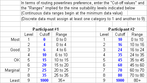
The questionnaire contains a series of statements that provide a consistent scale for calibrating the map layers. A calibration scale of 1 (least preferred) to 9 (most preferred) is used. The respondent identifies “cutoff values” for the data ranges for continuous mapped data and directly assigns ratings to map categories for discrete maps. It is critical that a consistent scale is applied independently to all maps and that each map contains at least one 9 (least preferred) and one 1 (most preferred) rating.

The questionnaire forms a series of questions soliciting cutoff values for continuous maps or direct rating assignments for discrete maps. A calibration question is developed for each map layer in the model. In the routing example, a question involving housing density (continuous) might be written as:

In terms of a preference to avoid areas of high housing density when routing electric transmission lines, what cutoffs for housing density are appropriate for the nine preference levels indicated below?

	Level	Cutoff	Implied Data Range
Most Preferred	1	________	________ to ________
	2	________	________ to ________
Good	3	________	________ to ________
	4	________	________ to ________
OK	5	________	________ to ________
	6	________	________ to ________
Marginal	7	________	________ to ________
	8	________	________ to ________
Least Preferred	9	________	________ to ________

Self-rated expertise level on this rating (1= low to 9=high) _____________

What constitutes the second round?

Working separately, the respondents enter map values for the “Cutoff” and “Implied Data Range” that define the nine preference levels for each question. While group discussion is encouraged in the first round, it is important that second round responses are completed independently to insure anonymity and avoid undue influence by dominant personalities. The self-rated expertise level indicated on each question can be used to derive weighted statistics useful in further discussion.

Note: The individual categories defining a discrete map are listed with a column for participants to record their preference level for each map category. Preference levels can be repeated but each map layer must contain a 1 (most preferred) and a 9 (least preferred) assignment.

How are the individual responses recorded at the completion of the second round?

Face-to-face group meetings are best, however a conference call coupled with online responses can be used if travel is impractical. In either case, the individual responses are recorded in a spreadsheet for statistical summary.

In the example, Participant #1’s cutoff values represent a much more stringent interpretation of housing density levels than Participant #2’s cutoff values.

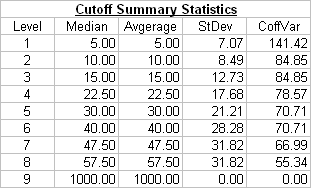
What information is in the controlled feedback from round 2?

In the example, the median and mean are the same as only two responses are considered. Note extremely high coefficient of variation (141.42) for the cutoff values assigned to preference level 1. This indicates an extreme difference of opinion in what housing density levels are most preferred (0 to 0 vs. 0 to 10 houses within 450m radius). The cutoff for the least preferred level 9 appears to be less contentious as its coefficient of variation is much lower (55.34).

Note: For discrete map ratings a similar set of statistics are calculated for each map category.

How are the final calibration ratings developed in the third round?

The statistical summary of the group’s responses serves a catalyst for further discussion. Each question is visited and the group discusses why a cutoff value should be higher or lower than the mean. The coefficient of variation is an indicator of the amount of compromise needed to reach consensus.

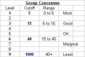
In many cases, group consensus is reached and final ratings can be directly assigned. If not, new response sheets for the questions in conflict are distributed and the participants are asked to re-enter their ratings based on the extended discussion. Members of the group expressing extreme views are asked to develop a brief written statement justifying their position. The process is repeated until an acceptable coefficient of variation is reached and the group mean is assigned, or a deadlock occurs.

In the example, group discussion decided to only identify four preference levels using the group means as the cutoff values defining the data ranges.

How are the derived calibration ratings used in a GIS model?

(Click image to enlarge) The cutoff values are used to reclassify the input maps in terms of the model’s objectives. In avoiding locations of high housing density, for example, densities from 0 to 5 houses are the most preferred (Preference Level 1) while densities greater than 40 houses are least preferred (Preference Level 9). The ratings for avoiding locations far from roads, locations close to sensitive areas and locations of high visual exposure are similarly used to calibrate the other map layers.

What are the benefits of using Delphi in calibrating GIS Models?

The most obvious benefit is the development of calibration ratings needed to implement a GIS model. Less obvious benefits surround the process itself. First, it engages a group of experts in structured discussion that insures all interpretations are presented. In addition, it documents group interactions leading to the calibration ratings. The result is a “consistent, objective and defendable” procedure for calibrating GIS models.