Applying MapCalc Map Analysis Software

Travel-Time and Customer Access: A market analyst needs to construct an “underlay” for a client’s MapInfo database that shows the travel-time from Kent’s Emporium to all other locations within a defined service area. This information will be invaluable in visualizing relative access of potential customers throughout the city.

<click here> for a printer friendly version (.pdf)

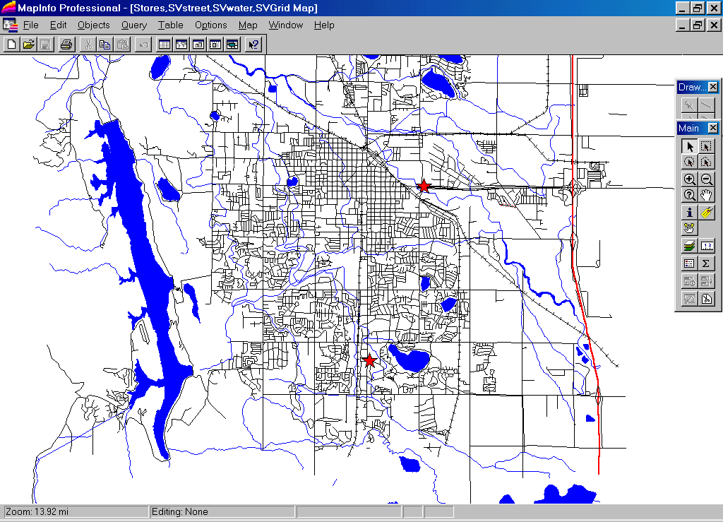
Base Maps. Standard MapInfo layers of streets, water and stores (Kent’s Place in the south and their major competitor Colossal Mart in the north) form the base layers for travel-time analysis.

Composite Display. Standard MapInfo layers of streets, water and stores (Kent’s Place in the south and their major competitor Colossal Mart in the north) form the base layers for travel-time analysis.

Step 1. The base maps in MapInfo are transferred to MapCalc for analysis.

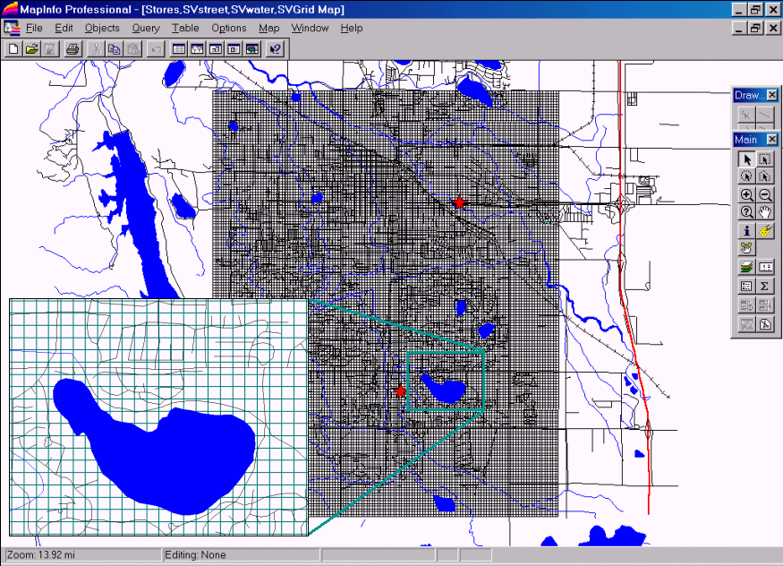
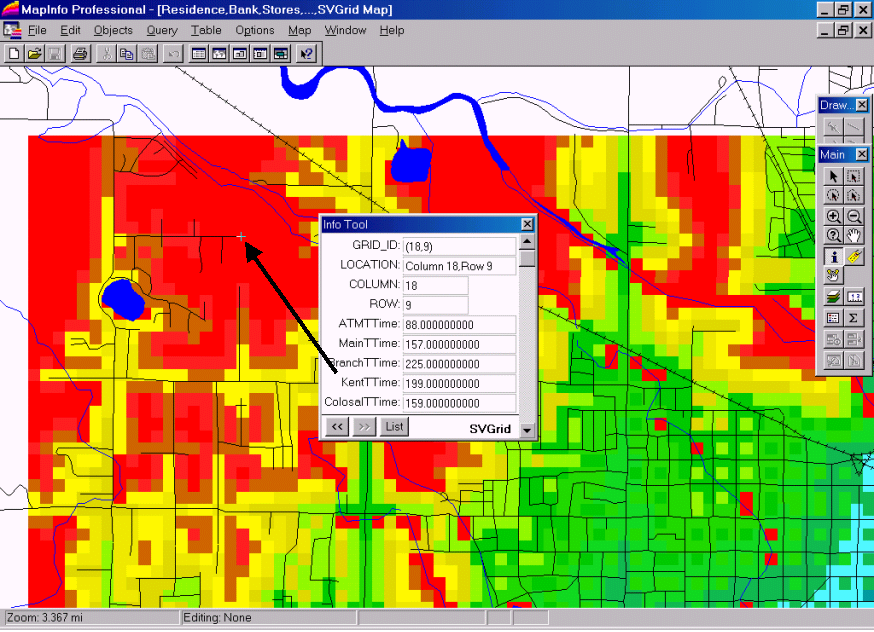
Pseudo Grid. A “pseudo grid” is constructed in MapInfo. Each grid cell is treated as a polygon forming 160 columns by 130 rows = 20,800 cells that comprise the analysis window. The insert in the lower left portion of the figure is an enlarged portion clearly showing the pseudo grid cells.

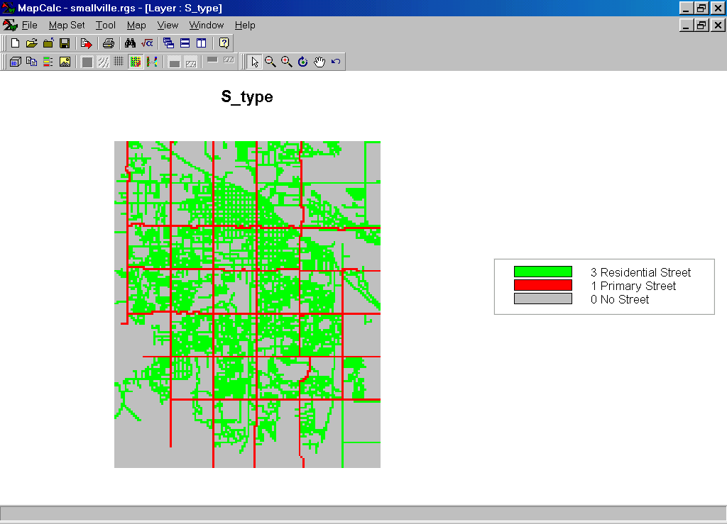S_type Map. Any MapInfo data layer (points, lines, polygons) can be “burned” into a similarly configured MapCalc analysis grid. For example, a grid-map of the MapInfo “streets” layer is imported into MapCalc. Each cell identifies whether a street is present with a separate value for the type of street (1= Primary Street…red; 3= Residential Street…green).

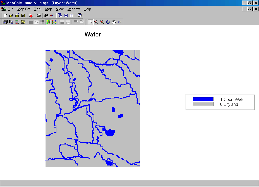Water Map. In a similar fashion, a grid-map of the water features is imported into MapCalc from MapInfo. The map identifies the presence of surface water (1= Open Water…blue).

Step 2. Using the proximity tool in MapCalc a travel-time distance is assigned to each of the 20,800 cells within the analysis window (see the “Proximity Demo” for discussion of how proximity surfaces are generated).

Kent’s_TTime Map. The travel-time values identify the quickest (shortest lapsed time) from Kent’s Emporium to all other locations respecting the inability to traverse open water (absolute barrier), the relative ease of travel along primary and secondary roads, and the much slower travel by walking where there are no roads (relative barriers). Note the bright red colored features that represent open water (streams and lakes) that are “infinitely” far away as they can’t be crossed by car or foot (without swimming). The dark blue identify areas that are very close to Kent’s Emporium. The spider web pattern reflects the relative ease of travel along the primary streets.

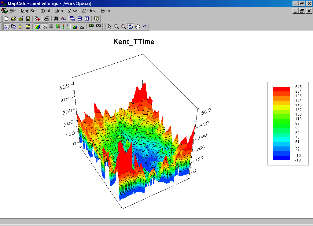
The 3-D surface on the right shows the increasing travel-time as a “bowl” with the lowest point being at the store (0 away from the store) and increasing time to all other locations. Note the big spikes indicating rapidly increasing travel-time for the non-road areas at the corners of the map. The southwest corner is the farthest away (545 units * 6 sec per unit= 3270 sec / 60 sec per min= 54.5 min by walking then by car along the fastest route).

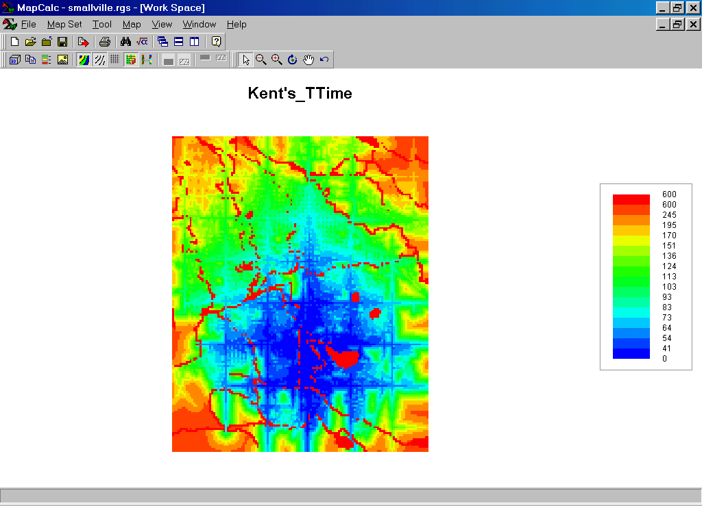
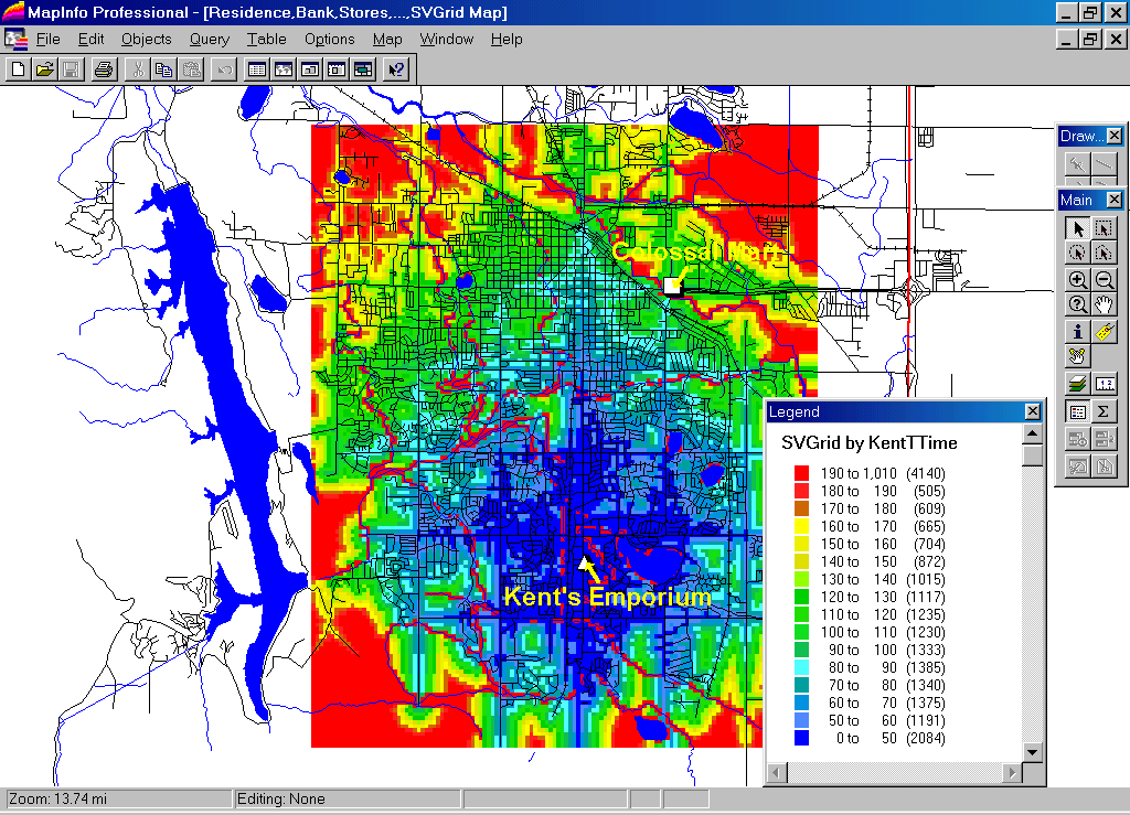
Step 3. The travel-time map generated in MapCalc is imported into MapInfo by appending the cell values to the pseudo grid table.

Kent’s_TTime Map (underlay). The detailed information appended from MapCalc to the pseudo grid is treated the same as any other MapInfo map. In this rendering it is themed into sixteen proximity ranges and used as a backdrop for the streets, water and stores maps.

The farthest away location on a street is nearly 20 minutes (199 units * 6 sec per unit= 1194 sec / 60 sec per min= 19.9 min). Potential customers on this street need strong motivation to visit the store.

Summary. Travel-time analysis is an important part of GIS technology but until recently grid-based tools have not been available in desktop mapping systems. Information exchange is easily accomplished between MapInfo and MapCalc by simply transferring maps between the matching pseudo grid and analysis grid in the respective systems. In addition to serving as graphical backdrops, the calculated values in MapCalc derived maps, such as viewsheds, population density and proximity maps, can be used in geoquery and advanced GIS models developed within MapInfo.

Note: A similar exchange of information between MapCalc and ArcView/ArcInfo users can be made. See the Determining Proximity application for discussion of the procedures used in calculating effective proximity.