Academic MapCalc: Educational Materials
for Instruction in Grid-Based Map Analysis
President, Berry & Associates //
Spatial Information Systems, Fort Collins , Colorado ,
USA
Kensinger, Jerry 2
Senior Software Engineer, Red Hen
Systems, Fort Collins , Colorado ,
USA
_____________________
Paper presented at the 15th Annual Conference on Geographic Information
Systems,
<click here>
for a printer friendly version (.pdf)
Abstract
Desktop mapping has gained popularity in many disciplines
across campus. The additional dimension
of “where” has provided new approaches to data analysis and decision
formulation. However, instruction in
grid-based processing has been limited.
Until recently,
Note: this
presentation contains several real-time demonstrations that are encapsulated in
several of the figures. A more complete
description of these and other grid-based processing examples are online at www.innovativegis.com/basis. The reader is encouraged to review the
examples then download a free evaluation copy of the MapCalc program from www.redhensystems.com for hands-on
experience and springboard to the Learner or Academic versions for more in
depth understanding of map analysis.
Introduction
Courses in Geographic Information Systems (
These vector-based systems are ideal for learning the
fundamentals of mapping and spatial database management. The educational experience with desktop
mapping provides an excellent entry into
Basic thematic mapping and geo-query, however, only address
a portion of
This paper describes some of the instructional considerations surrounding grid-based map analysis. In addition it describes the inexpensive MapCalc Learner software and supporting materials for student and instructor alike.
The Grid-Analysis Frame
Vector-based systems identify three basic map features that comprise all maps—points, lines and polygons. These features are suitable for characterizing discrete spatial objects, such as light poles, streets and property boundaries. However, continuous gradients, such as an elevation surface or a proximity map are poorly represented as contour lines that generalize detailed data into a set of intervals used for display.
The introduction of a grid-analysis frame provides a framework for storage and processing of a fourth basic map feature—a surface. The grid-based construct enables display and processing of geographic space as a continuum. Its base spatial unit is a cell defined by the column and row coordinates of an imaginary grid superimposed over an area. The base spatial unit is a grid cell and is used to identify…
· Points—single cell,
· Lines—connected set of cells,
· Polygons—all cells identifying the edge and interior of the parcel, and
· Surface—all cells within a project area with a value assigned to each that indicates the presence by feature type (discrete object) or the relative variable response (continuous gradient.
 Figure
1. The grid-analysis frame is used to
represent geographic space as a continuum.
Figure
1. The grid-analysis frame is used to
represent geographic space as a continuum.
The top left portion of figure 1 shows an elevation surface displayed as a traditional contour map, a superimposed analysis frame and a 2-D grid map. The highlighted portion of the table depicts the elevation value (1,635 feet) stored at one of the grid locations. The remainder of the table shows the values stored on other map layers at the same location. As the cursor is moved, the “drill-down” of values for different locations are instantly updated.
The plots in the lower portion of the figure show two types of 3-D displays. Connecting the grid lines at the center of each grid space forms a lattice structure. The lengths of the lines are a function of the difference between the values stored at adjacent grid spaces. The result is a “wireframe” that forms the peaks and valleys of the spatial distribution of the data. The color zones identify contour intervals that are draped on the frame.
The larger plot in the lower-right portion of the figure shows a grid structure surface of the same data. The boundary lines for each grid space are drawn to a relative height as function of the stored value. The result is a “stepped surface” that depicts the actual data defining the terrain and available for map analysis.
Map Analysis Procedures
An important characteristic of grid-based data is that a map area is subdivided into a uniform set of parcels (grid cells) that is used to characterize all map layers. The analysis frame provides the geographic consistency needed for investigating spatial relationships within and among grid layers. However the consistency is obtained at a loss in positional accuracy unless the grid is very fine and approaches the X,Y reference grid used in a vector-based system.
The tradeoff between positional accuracy and analysis utility is key in determining appropriate applications for vector and grid-based systems. In general, vector systems are best suited for computer mapping and geo-query of discrete map features but have limited map analysis capabilities. Grid systems, on the other hand, are ill suited for mapping and query but contain a robust set of analytical operations.
For example, consider calculation of terrain slope. In a vector-based system the relative distance between contour lines graphically portrays steepness—closer the lines the steeper slopes. But the ability to calculate a slope map is practically impossible using this data structure.
 Figure
2. Calculation of terrain slope and
surface flow maps.
Figure
2. Calculation of terrain slope and
surface flow maps.
The top portion of figure 2 shows 2-D and 3-D views of a slope map derived using the analysis frame. The larger 3-D display on the right shows the slope map draped over the elevation surface. Note that the steep areas (green) and flat areas (red) align with the appropriate surface inclinations providing visual conformation of the calculated slope values. As diagramed in the figure, the processing involves moving a 3x3 window over the entire elevation surface and calculating the slope of a plane that best fits the nine elevation values in the roving window.
The bottom portion of the figure shows a derived surface flow map. Note that the areas with higher flow values (green) align with the small ravines visible on the terrain surface. The process simulates a drop of rain falling at each grid cell, tracing its steepest downhill path while accumulating the number of paths that cross each cell. Higher numbers on the flow map indicate locations of water confluence.
Problem Solving
The result of an individual map analysis operation is the assignment of a computed value (slope and flow in the previous example) for every grid cell of a new map layer. Sequencing operations develop analysis procedures, such as erosion potential, as depicted in Figure 3.
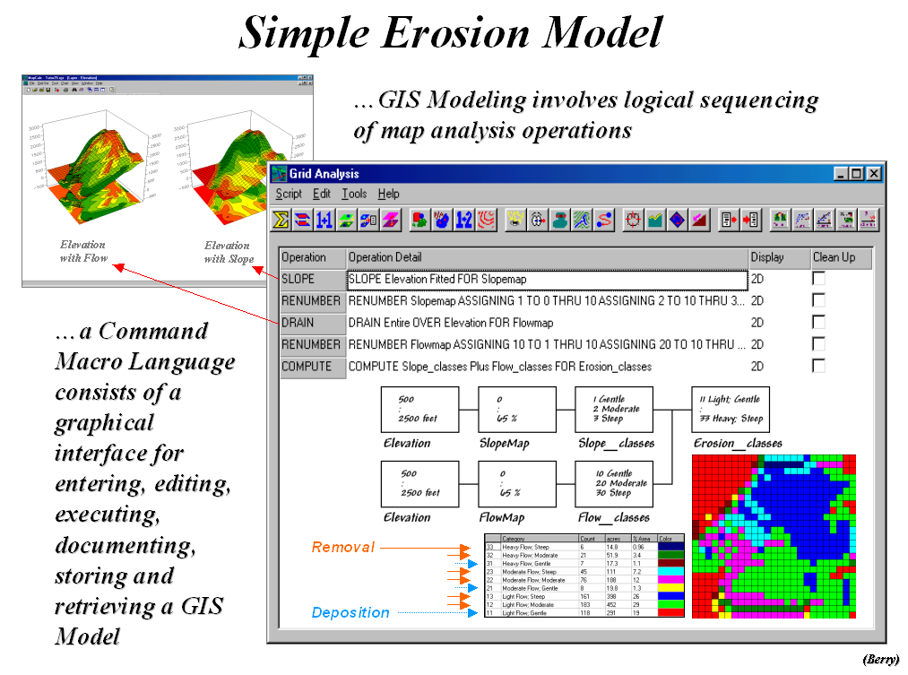 Figure 3. A command macro contains logically sequenced
map analysis operations that solve a problem.
Figure 3. A command macro contains logically sequenced
map analysis operations that solve a problem.
The two red arrows in the figure link the MapCalc commands with the 3-D displays of the slope and flow maps. Calibrating and combining the two maps construct a simple erosion potential model. Common sense suggests that areas with steep slopes and heavy flows tend to have higher erosion than flat areas with minimal flows.
The sequence of commands listed in the macro accomplishes three things—1) derives the slope and flow maps (using the SLOPE and DRAIN operations), 2) calibrates these layers for gentle-moderate-steep and light-moderate-heavy classes (RENUMBER), and 3) combines the two maps into a single erosion potential map (COMPUTE). The procedure used a simple mathematical trick where the slope classes are assigned the values 1, 2 and 3 while the flow classes are assigned 10, 20, and 30. Adding the two maps generates a two-digit code with the first number (tens digit) indicating the slope class and the second number (ones digit) indicating the flow class—e.g., 11 isn’t an eleven but a “one-one” depicting a location with a gentle slope (1) and a light flow (1).
The map in the lower-right corner shows all of the
combinations of slope and flow classes that occur in the project area. The color-coded arrows identify the
combinations as to whether erosion (orange) or deposition (blue) is likely to
occur. While this simple erosion model
is far from complete it has general merit and aptly illustrates the
construction of a command macro used to evaluate a
 Figure
4. Extending the simple erosion model.
Figure
4. Extending the simple erosion model.
Figure 4 diagrams an extension to the simple model that generates an effective proximity map to open water based on the intervening erosion potential. The RENUMBER operation is used to calibrate the map in figure 3 into a “friction” map characterizing the relative difficulty of erosion—1= high …10= minimal erosion potential. The SPREAD operation (dialog box in lower-left) is used to calculate effective distance from the streams and lakes on the water map. This process is like successive buffers in a vector-based system but the buffers reach farther in areas of high erosion potential—a “variable-width” buffer that is responsive to intervening conditions.
Consider the sketch in the top portion of the figure. A simple buffer of 250 feet on either side of the stream would allow soil-disturbing activities near the top of the steep inclination that would likely result in considerable sediment raining down on the stream. On the other side of the stream, activities would be prohibited although the terrain is perfectly flat and erosion potential minimal. A variable-width buffer, however, reaches much farther on the right side and much less on the left—not 250 feet regardless of conditions.
 Figure
5. Additional examples of
distance/connectivity operations (simple versus effective distance, optimal
paths, and visual exposure).
Figure
5. Additional examples of
distance/connectivity operations (simple versus effective distance, optimal
paths, and visual exposure).
Distance operations in MapCalc involve calculation of a series of concentric rings about a starting location (point feature) or set of locations (line or polygon feature). These rings are analogous to the ripples generated by tossing a rock into a pound—splash, one away, two away, etc. Every grid cell in the map area is assigned its “ripple number” with larger values indicating greater distances. When viewed as a 3-D plot, simple proximity forms a bowl-like accumulation surface about the feature (top-right plot in figure 5) with the starting locations of the water map forming the “valley” and increasing proximity forming the “mountains.”
Effective proximity considers the intervening conditions as the wave propagates. The result is a warped-bowl-shaped accumulation surface with varying slopes that correspond to changes in conditions. Steeper areas indicate locations that are effectively farther away than simple straight-line distance suggests.
Simple distance is defined as “the shortest, straight line between two points.” Simple proximity relaxes the limitation of just two points to “…among sets of locations,” such as all water cells to all other grid cells. Effective proximity further relaxes the assumption of straight-lines allowing distance measurement to simulate movement considering the effects of relative and absolute barriers. The ability to characterize realistic connectivity among map features and relax the oversimplifying assumptions of Euclidean geometry greatly extends simple buffer analysis in desktop mapping systems—“as-the-crow-flies.”.
But if straight-line connectivity is not assumed, the question arises what is the “shortest, not necessarily straight route connecting two points?” This involves optimal path analysis that tracks the steepest downhill path over an proximity surface. In effect, this process retraces the route the wave front took from the starting location(s) around and through the intervening barriers to any other location on the surface. Like walking through a parking lot with a lot of mud puddles you could choose to go around some and slowly trek through others. In effect accumulation surface analysis evaluates all possible routes and assigns the shortest—the value indicates the distance away and the optimal path indicates the route.
The concept of connectivity can be expanded to include visual connectivity by considering straight-rays in three-dimensional space. If the ridge occurs between two points one cannot be seen from the other. If the ray is not interrupted, the two points are visually connected. Grid-based visibility analysis, however, does not use vector calculations in three-dimensional space. It uses the distance “ripples” to identify the distance from a viewer location and calculates the difference in elevation to derive a “rise to run” ratio (tangent) between two points. If the ratio is larger than any of the ratios of the previous rings along the cell is marked as seen and that ratio becomes the one to beat as the wave front continues. In effect, the algorithm goes “splash” at a viewer cell and the wave front propagates carrying the tangent to be beat that is evaluated at each location as it is crossed.
The result is a map that identifies a viewer location’s viewshed—all locations that can be seen. If multiple viewer locations are considered a visual exposure surface is derived—map values indicate the number of times seen. If the viewer cells have differential weights a weighted visual exposure surface is generated. If the weights are both positive (beautiful things) and negative (ugly things) a net-weighted visual exposure surface is generated. For example, a recreation planner might generate such a map to use in locating a hiking trail that has the best views of beautiful features while avoiding visual connections to ugly things.
MapCalc
Educational Software and Materials
The discussion in the previous section illustrates just a few of the map analysis capabilities contained in MapCalc.
 Figure
6. Listing of MapCalc functions—map
analysis operations.
Figure
6. Listing of MapCalc functions—map
analysis operations.
The twenty-six analytical operations are grouped into five
classes—reclassify, overlay, distance, neighbors
and statistics—as listed in figure 6.
The previous discussions involved the analytical operations of SLOPE
(neighborhood), RENUMBER (reclassify), COMPUTE (overlay), DRAIN, SPREAD, and
RADIATE (distance). A cross-reference to
comparable operations in other grid-based systems is included in the
documentation. For example, the
translation to GRID commands (a module of ARCINFO
Command entry in MapCalc is made through pop-up dialog boxes similar to the one shown in the lower-right portion of figure 4. Each command forms a complete and grammatically correct English sentence that is added to the command macro log as it is executed. These macros can be edited, modified, and interleaved with descriptive notes then saved for re-execution. The use of an intuitive command language is ideally suited for teaching as complex programming languages often confuse and intimidate students with minimal computer expertise. Contextual help is available for all commands.
 Figure
7. Listing of MapCalc functions—map
display and summary.
Figure
7. Listing of MapCalc functions—map
display and summary.
In addition, there are over fifty “tools” for displaying maps, investigating data, charting, windowing, importing/exporting, and managing files (see figure 7). All interaction with the software is through graphical user interfaces and standard Windows icons including buttons, scroll lists, hot-fields, etc. The interface is designed so most interaction is completed through mouse-clicks with minimal keyboard entry. Data exchange includes most grid formats and popular desktop mapping files.
The MapCalc educational system comes in three forms—a free
download of the program, the MapCalc Learner package for students and the
MapCalc Academic for instructors. The
Learner CD contains the MapCalc and Surfer tutorial systems,
exercises/databases, application demos and two online texts—Map Analysis,
a compilation of Dr. Berry’s “Beyond Mapping” column in GEOWorld and Precision
Farming Primer, a compilation of his “Inside the
 Figure
8. Listing of materials in the MapCalc
Learner and Academic packages.
Figure
8. Listing of materials in the MapCalc
Learner and Academic packages.
The MapCalc software by Red Hen Systems (www.redhensystems.com) has extensive capabilities
in spatial analysis and statistics. The Surfer
software by Golden Software (www.goldensoftware.com)
provides extended capabilities in surface modeling and 3-D graphics. The MapCalc tutorial version is constrained
to a 100x100 grid configuration (10,00 grid cells) and some of Surfer’s output
features are constrained in the tutorial version. Both software systems have data exchange
tools and accept data for creating your own databases.
The MapCalc Learner package is designed for
student and self-learning and licensed for educational use on a single
computer. It is distributed on a single
CD for US$21.95 plus shipping and handling.
The MapCalc Academic package is designed for instructors and contains
all of the Learner materials plus lecture PowerPoint’s, additional exercises,
one-day workshop and full introductory course materials supporting classroom
instruction. The materials were
developed by Dr.
Conclusion
The discussion in the “Problem Solving” section of this
paper illustrates a small set of the analytical operations in grid-based map
analysis. The live demonstrations and
online annotated applications provide a wealth of experience in
In many respects
The MapCalc educational materials enable students and
instructors an opportunity to get hands-on experience in applying this powerful
yet often overlooked side of
__________________________
1Joseph K. Berry is the President of
Berry & Associates // Spatial Information Systems, consultants and software
developers in
2Jerry Kessinger is a Senior Software
Engineer with Red Hen Systems, a systems development company specializing in
multimedia mapping and data processing for site-specific agriculture. Contacts: Red Hen Systems, 2310 E. Prospect
Road, Suite A