Applying MapCalc Map Analysis Software

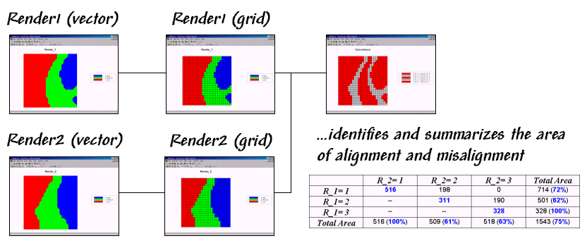
Comparing Discrete Maps (Coincidence Summary): A geographer wants to compare two interpreted maps of the same area and quantitatively report how similar they are.

<click here> for a printer friendly version (.pdf)

Processing Flow.

Base Maps. The Base Maps needed include:

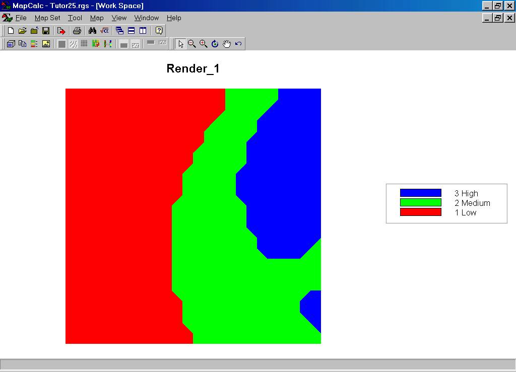
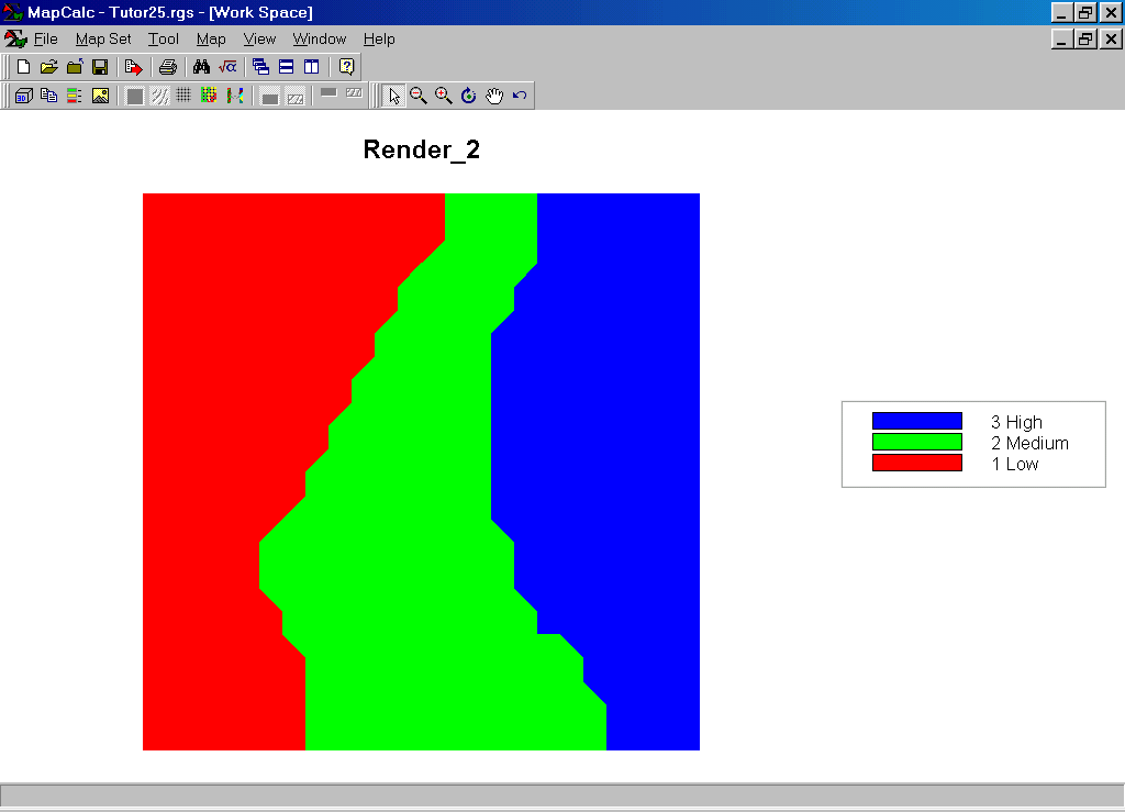
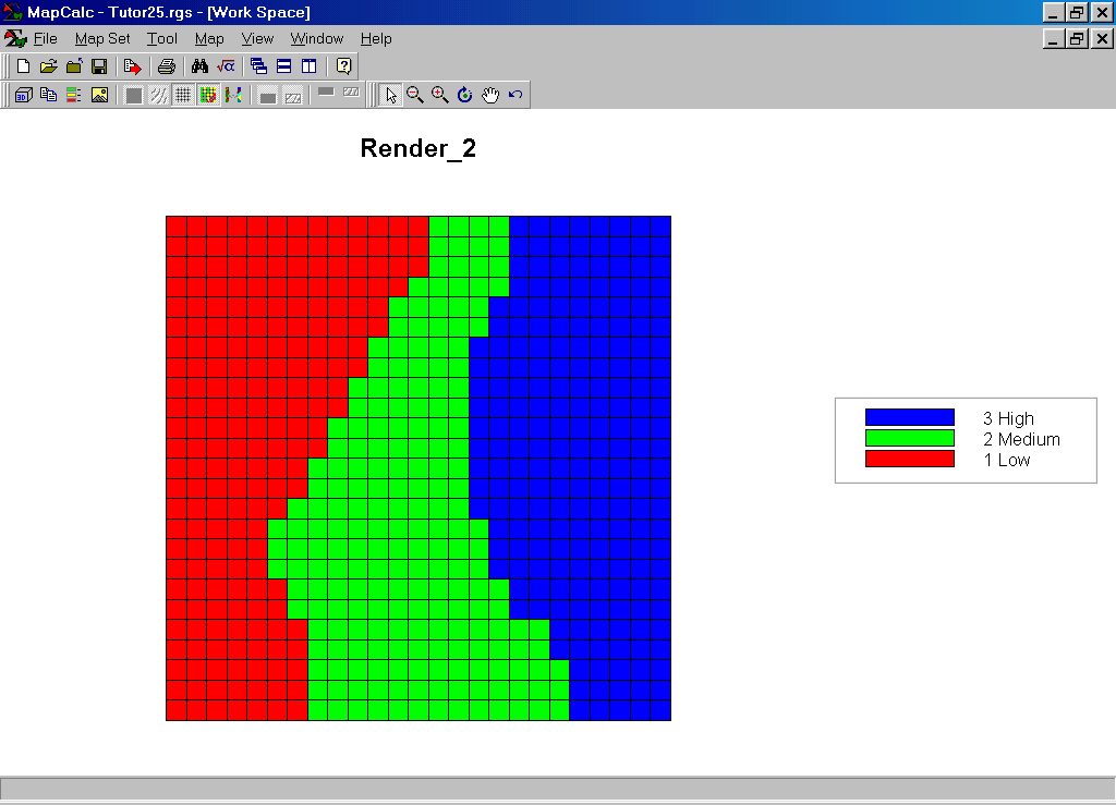
Renderings 1 and 2. The two maps appear quite similar— or maybe quite dissimilar… what’s your call? Visual comparison is subjective and difficult to standardize.

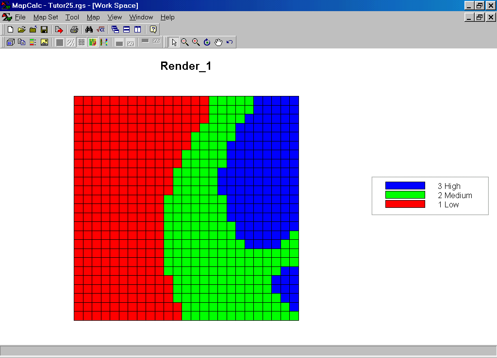
Grid Maps. The two contour maps are converted to grid maps for analysis.

Step 1. The MapCalc operation…

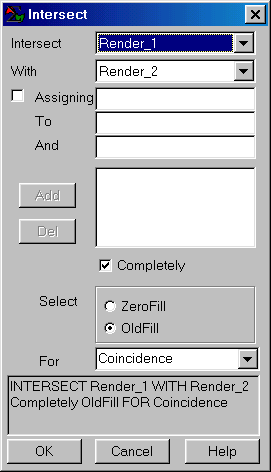INTERSECT Render_1 WITH Render_2 Completely FOR Coincidence.

…generates a map that identifies the “joint condition” at each location.

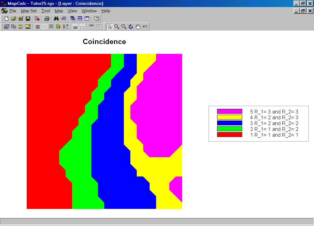
Coincidence Map. The coincidence of the two maps resulted in five categories—three indicating identical map assignments (map values 1, 3 and 5) and two with mixed assignments (map values 2 and 4).

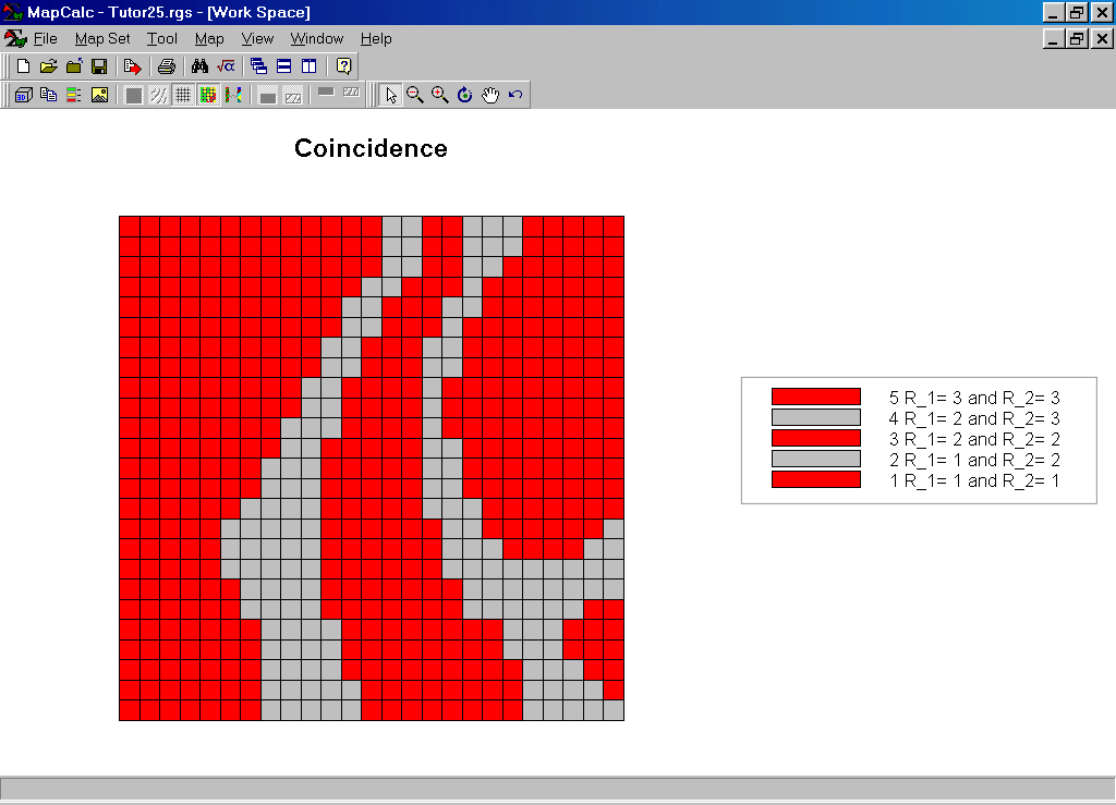
Agreement/Disagreement Display. MapCalc’s shading manager was used to reassign red to areas identifying locations that had the same classification on both maps— agreement. The gray areas identify locations with different classifications— disagreement. If the two maps were identical the entire map display would be red. Increasing amounts of gray indicate differences between the renderings. All gray would indicate totally dissimilar maps.

	R_2= 1	R_2= 2	R_2= 3	Total Area
R_1= 1	516	198	0	714 (72%)
R_1= 2	--	311	190	501 (62%)
R_1= 3	--	--	328	328 (100%)
Total Area	516 (100%)	509 (61%)	518 (63%)	1543 (75%)

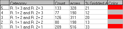
Coincidence Summary Table. This table summarizes the relative area within each coincidence combination. The diagonal entries indicate agreement while the off-diagonal entries indicate disagreement. The percentages indicate the relative amount of agreement for each category on the two maps— rows for the Render_1 map and columns for the Render_2 map. The percentage in the lower right corner reports the overall agreement between the two maps… ((516 + 311 + 328) / 1543) * 100= 75%.

Summary. The overall percent agreement statistic is a general indicator of the similarity between two discrete maps. The coincidence table contains information about the alignment for each category. The coincidence map identifies the spatial pattern of the alignment for each category and can be redisplayed with a color pallet that simply identifies overall agreement and disagreement. The procedure is useful in a variety of applications that need to compare discrete maps— e.g., change detection for vegetation maps from two different dates or the level of “interpreter’s license” for two different photo interpreters renderings of the same area… where do they agree; where do they disagree.

Note: The Render_1 and Render_2 maps are discrete contour maps derived from the same map surface…

Render_1 is a three interval, equal range classification of the Tutor25 Elevation surface:

RENUMBER Elevation ASSIGNING 1 TO 500 THRU 1170

ASSIGNING 2 TO 1170 THRU 1840

ASSIGNING 3 TO 1840 THRU 2500 FOR Render_1

Render_2 is a three interval, equal count classification of the Tutor25 Elevation surface:

RENUMBER Elevation ASSIGNING 1 TO 500 THRU 870

ASSIGNING 2 TO 870 THRU 1610

ASSIGNING 3 TO 1610 THRU 2500 FOR Render_2