Applying MapCalc Map Analysis Software
Generating Surface Maps from Point Data: A farmer wants to generate a set of maps
from soil samples he has been collecting for several years. Previously, he would simply calculate the average
of the sample values for each soil variable, such as amount phosphorous, and
develop a fertilization plan assuming the average level was everywhere the same
within a field. Creating surface maps of
these data enables him to visualize the spatial distribution of data as contour
and 3D displays. He also wants to
analyze the spatial patterns within the data (e.g., determine where in the
field there are unusually high or low amounts) and relationships among the maps
(e.g., determine where the greatest increase or decrease in a soil nutrient has
occurred over the past several years).
<click
here> for a printer friendly
version (.pdf)
What Is Surface Modeling? “Surface Modeling” involves developing a continuous surface from point-sampled data—in effect, filling-in areas without information based on set of surrounding point samples. When the result is displayed as a contour map the procedure is termed “contouring.” The process uncovers the spatial distribution inherent in the samples and is useful in identifying areas that have generally high or low responses. This information is valuable for a wide-variety of applications, such as determining areas of high animal activity, air pollution concentrations and market value pockets. Surface modeling has been used since the 1950s in generating temperature and barometric maps, but is only recently being applied to other data.
Basic Steps in Creating Surface Maps. There are three basic steps when using MapCalc to generate map surfaces…
- Step 1 – specifies the configuration of the analysis grid set (grid size, boundary and geographic registration)
- Step 2 – specifies the sample data for spatial interpolation
- Step 3 – specifies the interpolation technique to be used.
These steps are completed using the “Map Creation Wizard” that guides the user through a logical series of dialog boxes in which the user completes the required and custom “hotfields.” The entire process usually takes less than a minute.
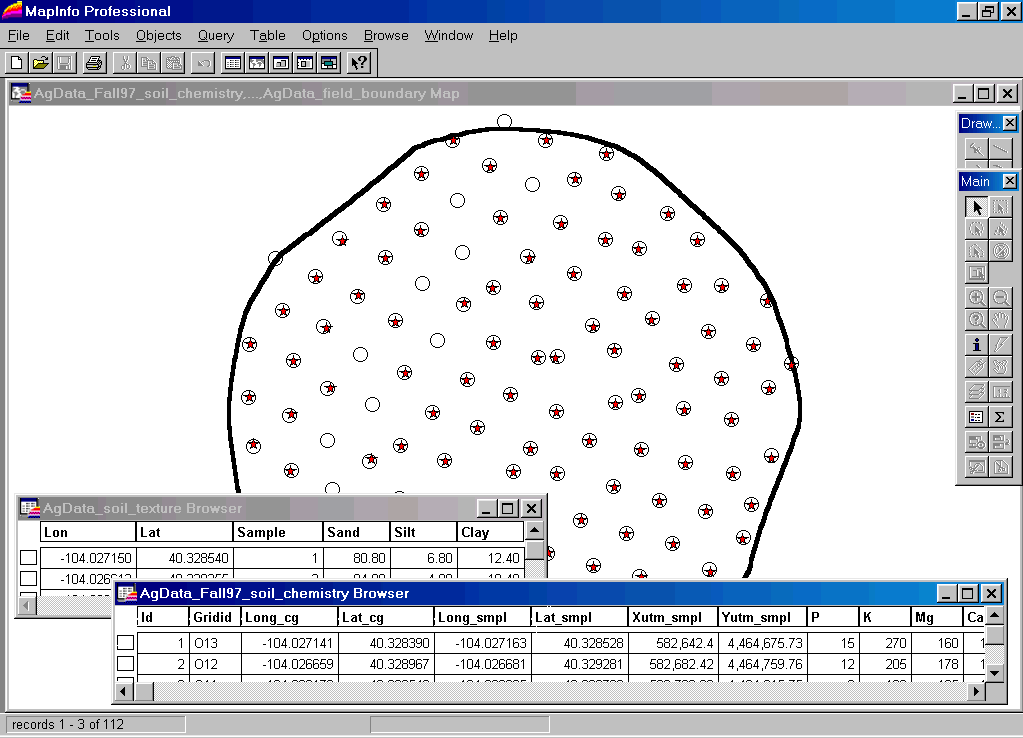 Step 0. The point data is stored in a general-purpose
desktop mapping system, such as ArcView (.shp file) or MapInfo (.tab
file) in this example. The “red stars”
indicate the location of soil chemistry samples and the “black circles”
indicate soil texture samples. The
underlying tables for each point map contains the sample data. The “black line” identifies the field
boundary.
Step 0. The point data is stored in a general-purpose
desktop mapping system, such as ArcView (.shp file) or MapInfo (.tab
file) in this example. The “red stars”
indicate the location of soil chemistry samples and the “black circles”
indicate soil texture samples. The
underlying tables for each point map contains the sample data. The “black line” identifies the field
boundary.
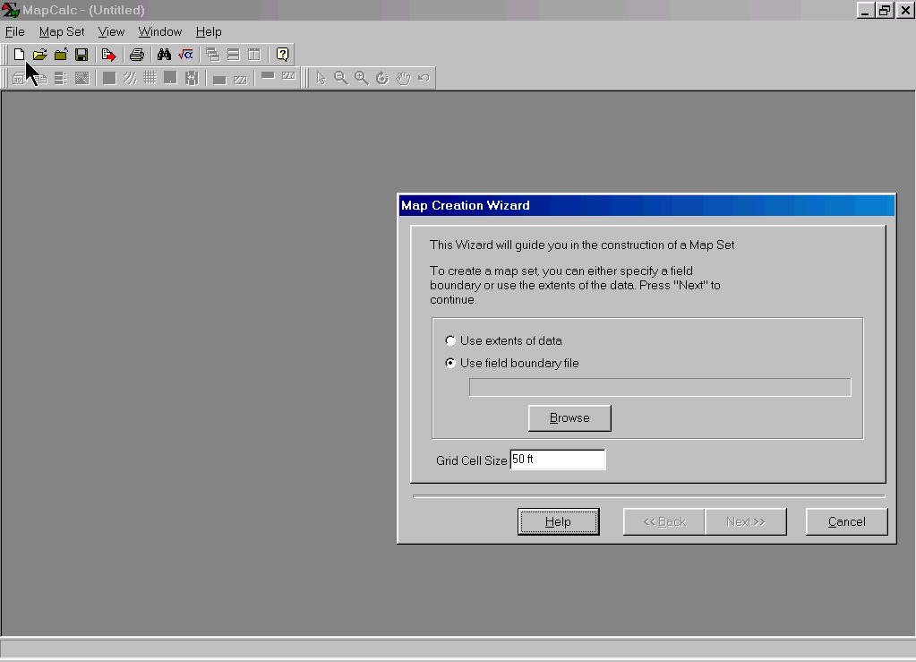 Step 1a. Access MapCalc and press the Create a
new file button on the main menu bar to pop-up the first dialog box in
the “Map Creation Wizard.” Enter the
appropriate Grid Cell Size (50 feet), select Use Field Boundary
File, and press the Next button.
Step 1a. Access MapCalc and press the Create a
new file button on the main menu bar to pop-up the first dialog box in
the “Map Creation Wizard.” Enter the
appropriate Grid Cell Size (50 feet), select Use Field Boundary
File, and press the Next button.
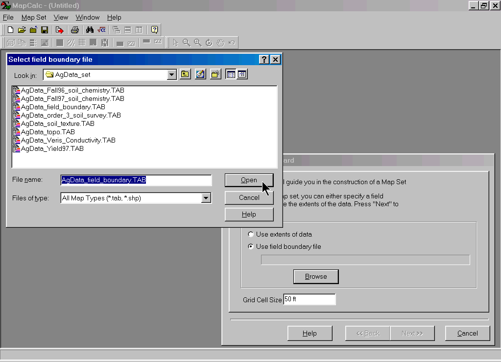 Step 1b. Navigate to and select the appropriate field
boundary file (AgData_field_boundary.tab), then press the Open
button and Next to advance to the dialog box.
Step 1b. Navigate to and select the appropriate field
boundary file (AgData_field_boundary.tab), then press the Open
button and Next to advance to the dialog box.
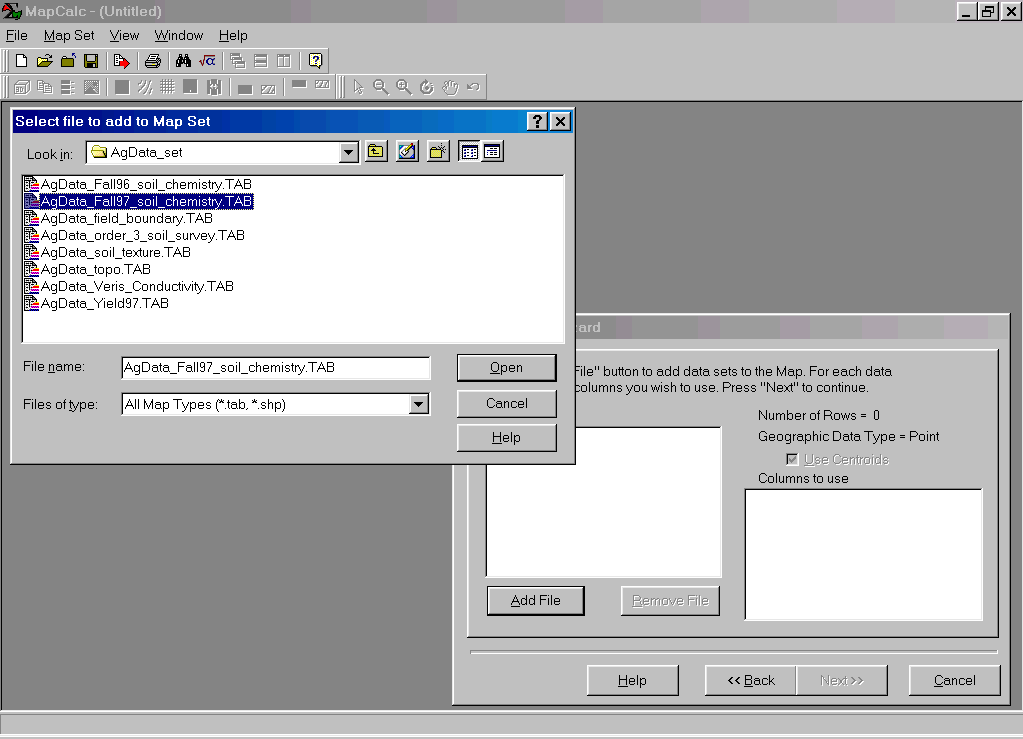 Step 2a. Press the Add File button and
navigate to the table containing the sample data (AgData_Fall97_Soil_chemistry.tab). Press Open to open the sample
data file.
Step 2a. Press the Add File button and
navigate to the table containing the sample data (AgData_Fall97_Soil_chemistry.tab). Press Open to open the sample
data file.
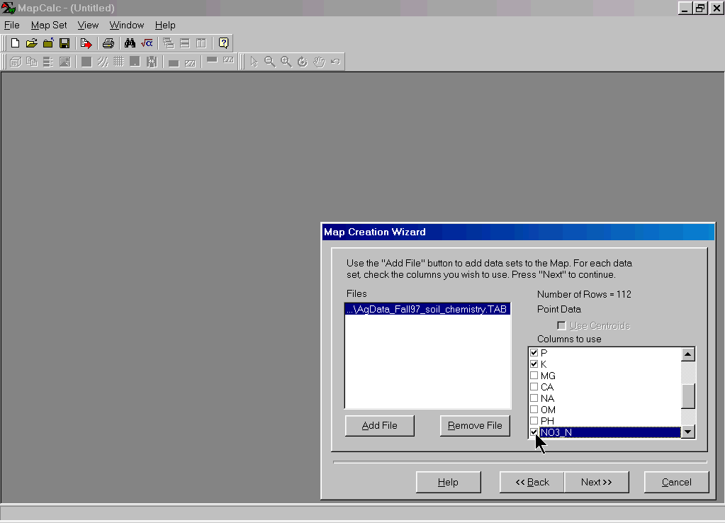 Step 2b. Select the sample data you want to map (P
<phosphorous>, K <potassium>, NO3_N <nitrogen>) and
press the Next button.
These specifications identify the “data fields” (columns) in the sample
data table that will be used—the X,Y (Longitude, Latitude) positions each data
point and the measure value reports the results of chemical analysis for each
soil sample. These “Discrete Point” data
serve as input to the spatial interpolation calculations to generate a
“Continuous Map Surface.”
Step 2b. Select the sample data you want to map (P
<phosphorous>, K <potassium>, NO3_N <nitrogen>) and
press the Next button.
These specifications identify the “data fields” (columns) in the sample
data table that will be used—the X,Y (Longitude, Latitude) positions each data
point and the measure value reports the results of chemical analysis for each
soil sample. These “Discrete Point” data
serve as input to the spatial interpolation calculations to generate a
“Continuous Map Surface.”
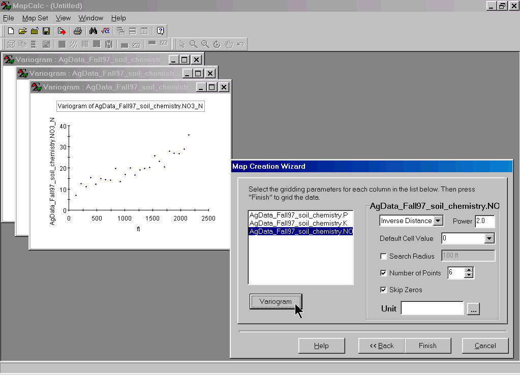 Step 3a. Specify the spatial interpolation technique (Inverse
distance Squared or Kriging) and the appropriate parameters (see
the MapCalc Manual for more information).
Highlighting a map name and pressing the Variogram button
generates a plot characterizing the spatial autocorrelation in the data. Generally speaking, a horizontal (flat) variogram
indicates minimal information for interpolation and the map surface generated
may be of negligible value. A variogram
exhibiting a tightly-clustered linear pattern suggests better map surfacing
results (see the MapCalc Manual for more information). Press the Finish button to
generate the map surfaces of the data fields you selected.
Step 3a. Specify the spatial interpolation technique (Inverse
distance Squared or Kriging) and the appropriate parameters (see
the MapCalc Manual for more information).
Highlighting a map name and pressing the Variogram button
generates a plot characterizing the spatial autocorrelation in the data. Generally speaking, a horizontal (flat) variogram
indicates minimal information for interpolation and the map surface generated
may be of negligible value. A variogram
exhibiting a tightly-clustered linear pattern suggests better map surfacing
results (see the MapCalc Manual for more information). Press the Finish button to
generate the map surfaces of the data fields you selected.
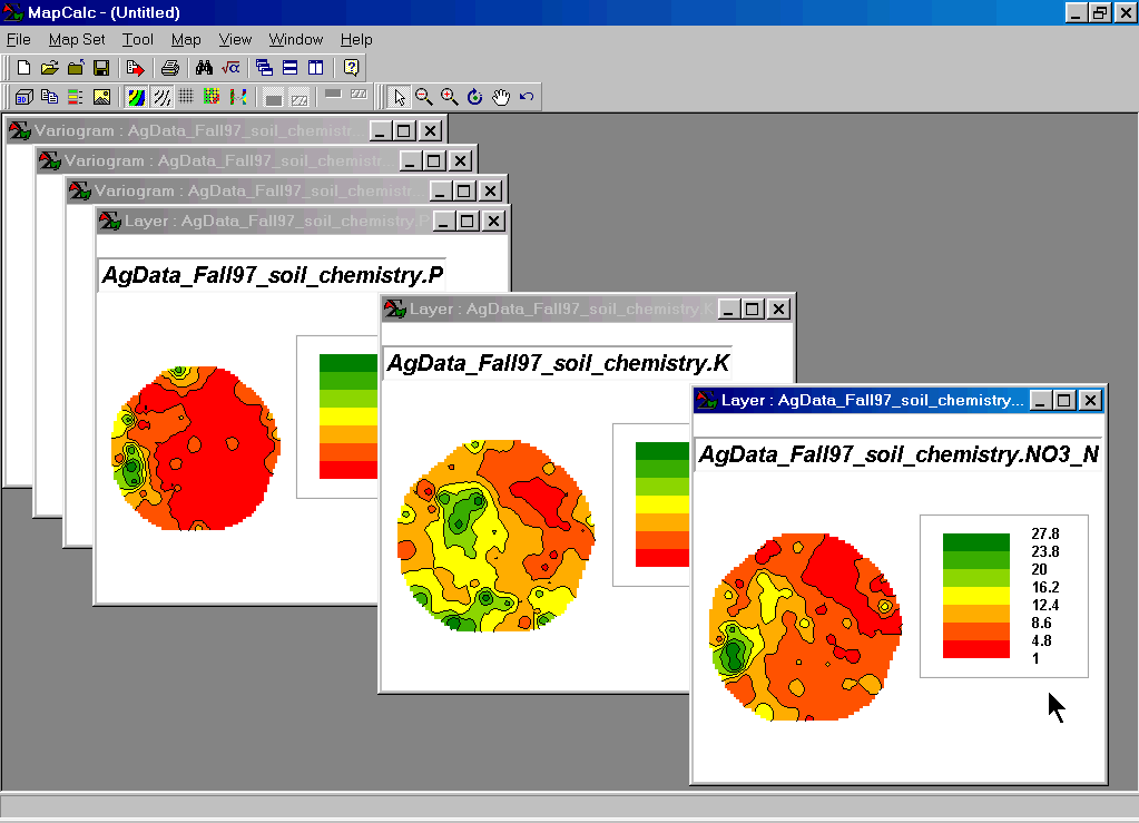 Step 3b. The map surfaces will be automatically
displayed in separate windows. These
maps can be displayed and evaluated with any of the MapCalc tools.
Step 3b. The map surfaces will be automatically
displayed in separate windows. These
maps can be displayed and evaluated with any of the MapCalc tools.
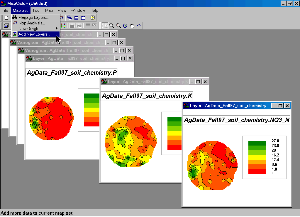 Step 4a. To add additional map layers to the current
database click Map Set à Add New Layers
from the main menu.
Step 4a. To add additional map layers to the current
database click Map Set à Add New Layers
from the main menu.
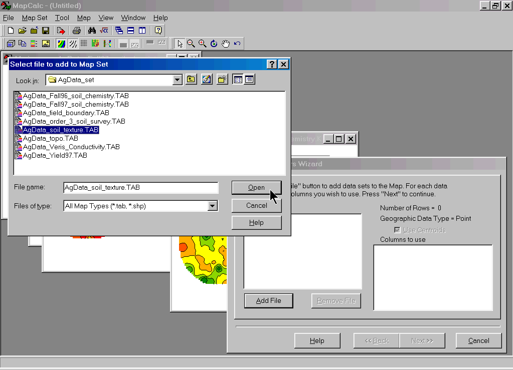 Step 4b. Navigate to the table containing the sample
data (AgData_ Soil_texture.tab).
Press Open to open the sample data file.
Step 4b. Navigate to the table containing the sample
data (AgData_ Soil_texture.tab).
Press Open to open the sample data file.
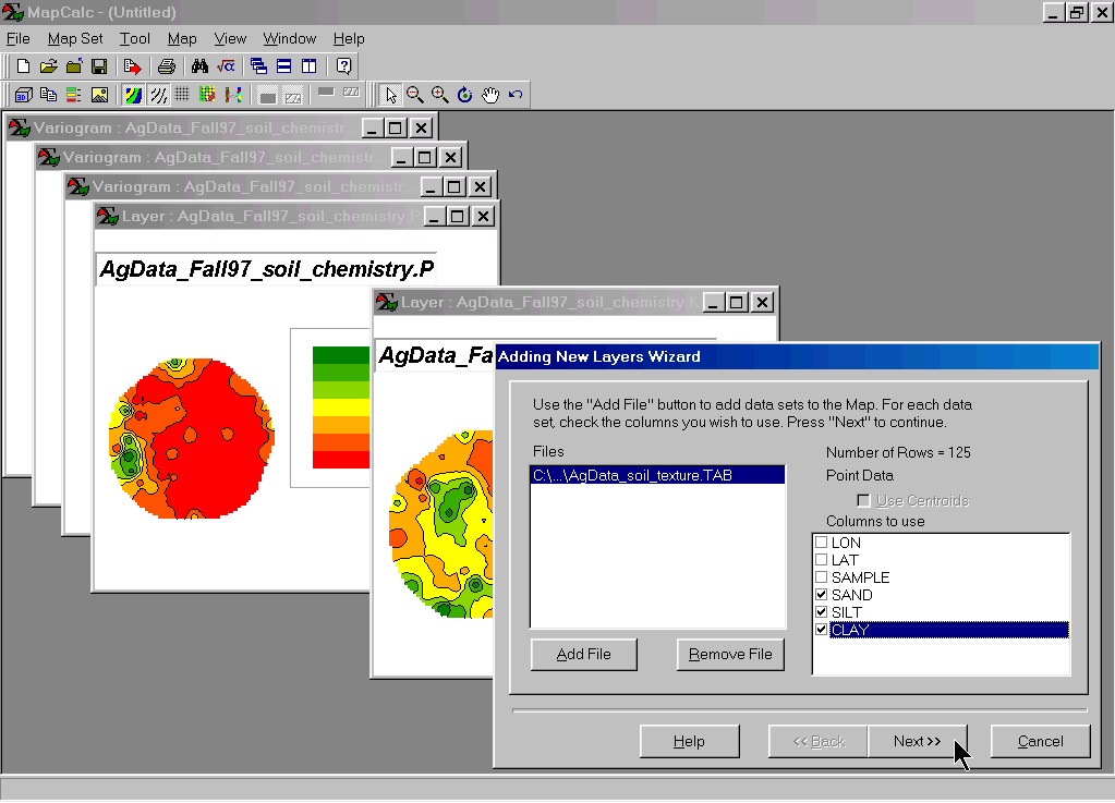 Step 4c. Select the sample data you want to map (Sand,
Silt and Clay) and press the Next button.
Step 4c. Select the sample data you want to map (Sand,
Silt and Clay) and press the Next button.
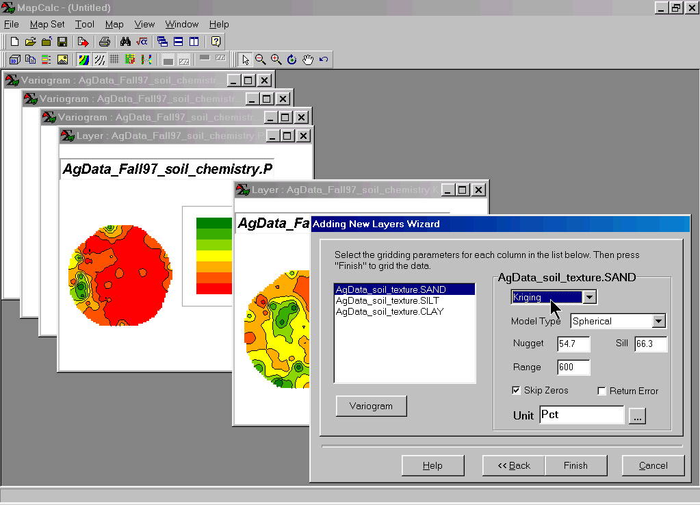 Step 5a. Specify the spatial interpolation technique (Inverse
distance Squared or Kriging) and the appropriate parameters. Generate and review the Variogram
plots for the data. Press the Finish
button to generate the map surfaces of the data fields you selected.
Step 5a. Specify the spatial interpolation technique (Inverse
distance Squared or Kriging) and the appropriate parameters. Generate and review the Variogram
plots for the data. Press the Finish
button to generate the map surfaces of the data fields you selected.
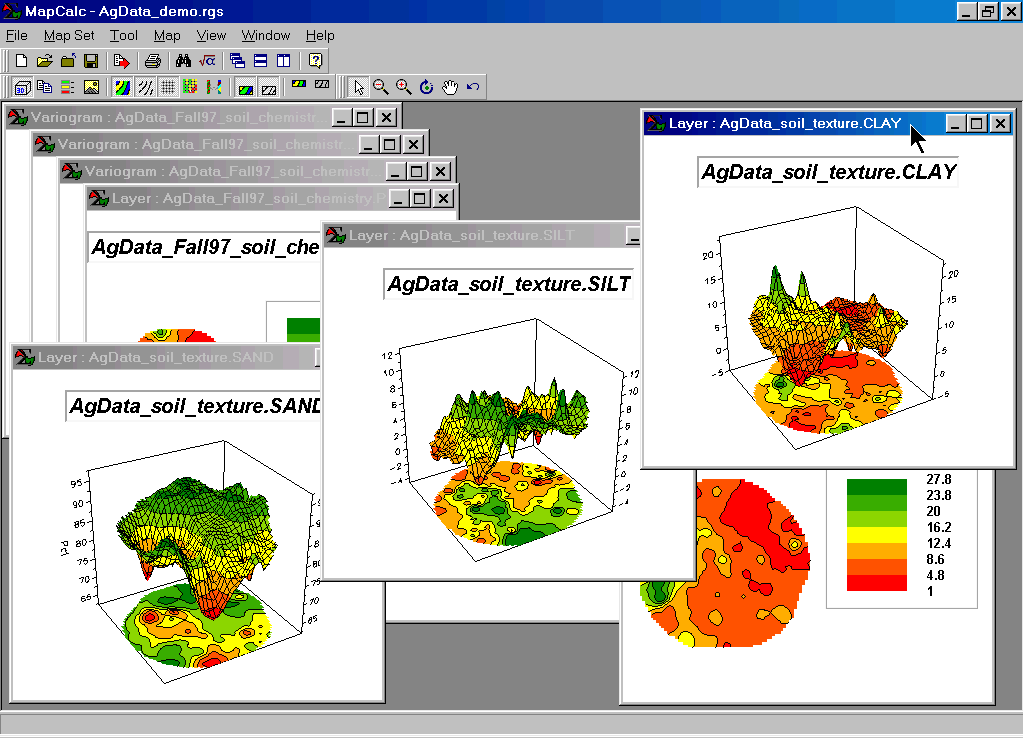 Step 5b. The map surfaces will be automatically
displayed in separate windows (switched to 3D lattice view).
Step 5b. The map surfaces will be automatically
displayed in separate windows (switched to 3D lattice view).
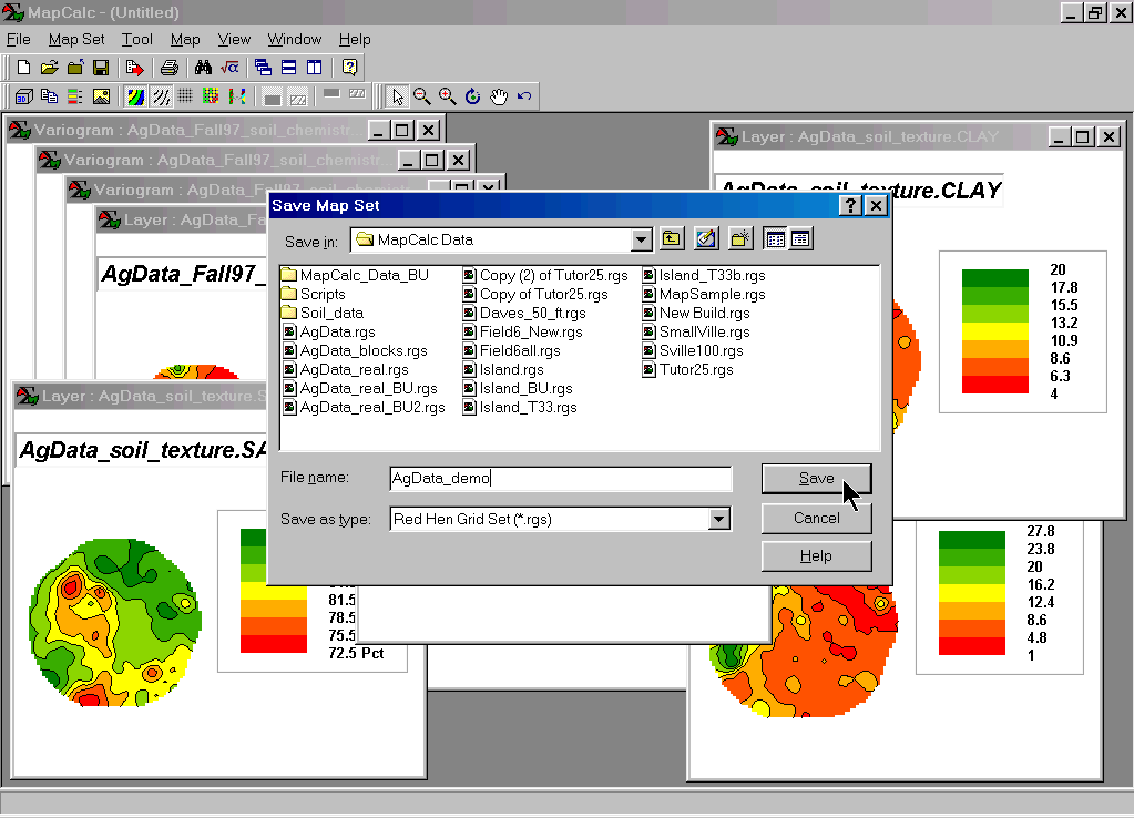 Step 6. Click Fileà
Save As from the main menu then navigate to an appropriate folder and
save the map with an appropriate name (AgData_demo.rgs).
Step 6. Click Fileà
Save As from the main menu then navigate to an appropriate folder and
save the map with an appropriate name (AgData_demo.rgs).
Summary. Surface modeling provides a powerful new perspective on most data collected in geographic space. Non-spatial analysis seeks to determine the “typical” value (average or mean) in a data set and assumes there are no spatial patterns. Spatial analysis, on the other hand, seeks to identify spatial patterns and use this information to explain relationships within and among data sets. In a sense, surface modeling “maps the variation in the data” and focuses attention on those areas that are not typical. In this example, the continuous surface maps of soil chemistry and texture can be used to develop a site-specific fertilization program that puts the appropriate amount of fertilizer at each map location based on the existing concentrations and texture conditions. The old method merely calculates the average concentration and texture condition for the entire field and develops a “typical” fertilization program that is applied everywhere the same. The ability to spatially tailor management actions based on point samples promises to revolutionize decision-making in many disciplines.