Applying Spatial Analysis and Surface
Modeling
in Decision-Making Contexts
Joseph K. Berry1
Berry & Associates, Suite 300,
2000 South College Avenue, Fort Collins, Colorado 80525
Phone: (970) 215-0825 — E-mail: jberry@innovativegis.com — Web site: www.innovativegis.com/basis
Abstract
The
characterization of terrain is an important aspect in sound land and resource
planning and management. Many
commercial GIS systems provide grid-based analysis tools that can be applied to
spatial analysis and surface modeling.
This paper describes several basic procedures for analyzing
micro-terrain characteristics: 1) Deviation from Trend, Difference
Maps and Deviation Surfaces to identify convex and concave features,
2) Coefficient of Variation Surfaces statistically summarizing disparity
in neighboring elevation values, 3) Slope and Aspect Maps that
report the magnitude and direction of surface inclination, 3) Slope of a
Slope Map (2nd derivative) that summarizes the frequency of the
slope changes, and 4) Confluence Maps characterizing the number of
uphill locations connected to each surface location. These tools provide a wealth of different perspectives on surface
configuration that are useful in decision-making in a wide variety of geo-based
applications.
Characterizing
Micro-Terrain Features
As
you look at a landscape you easily see the changes in terrain with some areas
bumped up (termed convex) and others pushed down (termed concave). But how can a computer "see" the
same thing? Since its world is digital,
how can the lay of the landscape be transferred into a set of drab numbers?
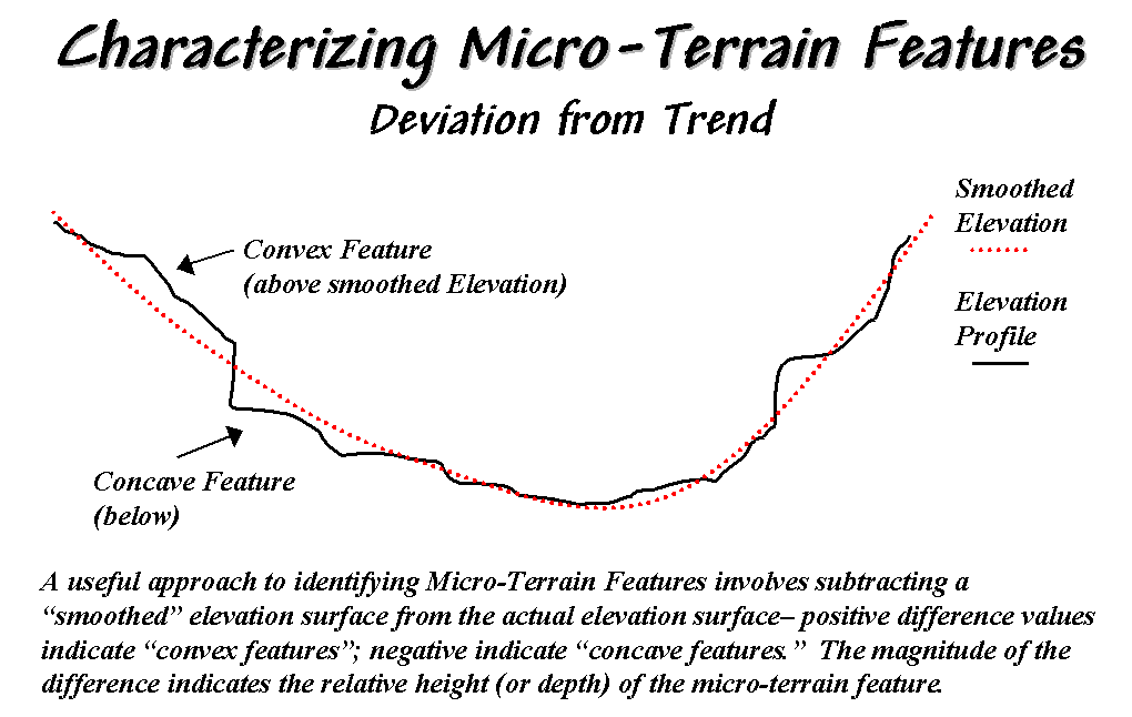 Figure 1. Identifying Convex and Concave features by
deviation from the trend of the terrain.
Figure 1. Identifying Convex and Concave features by
deviation from the trend of the terrain.
One
of the most frequently used procedures involves comparing the trend of the
surface to the actual elevation values.
Figure 1 shows a terrain profile extending across a small gully. The dotted line identifies a smoothed curve
fitted to the data, similar to a draftsman's alignment of a French curve. It "splits-the-difference" in the
succession of elevation values—half above and half below. Locations above the trend line identify
convex features while locations below identify the concave ones. The further above or below determines how
pronounced the feature is.
In
a GIS, simple smoothing of the actual elevation values derives the trend of the
surface. The left side of figure 2
shows the actual and smoothed surfaces for a project area. The flat portion at the extreme left is an
area of open water. The terrain rises
sharply from 500 feet to 2500 feet at the top of the hill. Note the small "saddle" (elevation
dips down then up) between the two hilltops.
Also note the small depression in the relatively flat area in the
foreground (SW) portion.
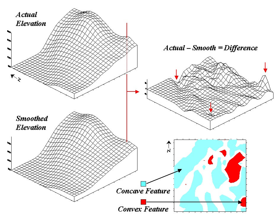 Figure 2. Example of a micro-terrain deviation
surface.
Figure 2. Example of a micro-terrain deviation
surface.
In
generating the smoothed surface, elevation values were averaged for a 4-by-4
window moved throughout the area. Note
the subtle differences between the surfaces—the tendency to pull-down the
hilltops and push-up the gullies.
While
you see (imagine?) these differences in the surfaces, the computer quantifies
them by subtracting. The difference
surface on the right contains values from -84 (prominent concave
feature) to +94 (prominent convex feature).
The big bump on the difference surface corresponds to the smaller
hilltop on elevation surface. It's actual
elevation is 2016 while the smoothed elevation is 1922 resulting in 2016 - 1922
= +94 difference. In micro-terrain
terms, this area is likely drier that its surroundings as water flows away from
it.
The
other arrows on the surface indicate other interesting locations. The "pockmark" in the foreground
is a small depression (764 - 796 = -32 difference) that is likely wetter as
water flows into it. The "deep
cut" at the opposite end of the difference surface (539 - 623 = -84)
suggests a prominent concavity. However
representing the water body as fixed elevation isn't a true account of terra
firma configuration and misrepresents the true micro-terrain pattern.
In
fact the entire concave feature in the upper left portion of 2-D representation
of the difference surface is suspect due to its treatment of the water body as
a constant elevation value. While a
fixed value for water on a topographic map works in traditional mapping
contexts it's insufficient in most analytical applications. Advanced GIS systems treat open water as
"null" elevations (unknown) and "mirror" terrain conditions
along these artificial edges to better represent the configuration of solid
ground.
The
2-D map of differences identifies areas that are concave (dark red), convex
(light blue) and transition (white portion having only -20 to +20 feet difference
between actual and smoothed elevation values).
If it were a map of a farmer's field, the groupings would likely match a
lot of the farmer's recollection of crop production—more water in the concave
areas, less in the convex areas.
Putting
Terrain Information to Use
A
Colorado dryland wheat farmer knows that some of the best yields are in the
lowlands while the uplands tend to "burn-out." A farmer in Louisiana, on the other hand,
likely see things reversed with good yields on the uplands while the lowlands
often "flood-out." In either
case, it might make sense to change the seeding rate, hybrid type, and/or
fertilization levels within areas of differing micro-terrain conditions.
The
idea of variable rate response to spatial conditions has been around for
thousands of years as indigenous peoples adjusted the spacing of holes they
poked in the ground to drop in a seed and a piece of fish. While the mechanical and green revolutions
enable farmers to cultivate much larger areas they do so in part by applying
broad generalizations of micro-terrain and other spatial variables over large
areas. The ability to continuously
adjust management actions to unique spatial conditions on expansive tracks of
land foretells the next revolution.
Investigation
of the effects of micro-terrain conditions goes beyond the farm. For example, the Universal Soil Loss
Equation uses "average" conditions, such as stream channel length and
slope, dominant soil types and existing land use classes, to predict water runoff
and sediment transport from entire watersheds.
These non-spatial models are routinely used to determine the feasibility
of spatial activities, such as logging, mining, road building and housing
development. While the procedures might
be applicable to typical conditions, they less accurately track unusual
conditions clumped throughout an area and provide no spatial guidance within
the boundaries of the modeled area.
GIS-based
micro-terrain analysis can help us be more like a "modern ancient
farmer"— responding to site-specific conditions over large expanses of the
landscape. Calculation of a difference
surface simply scratches the surface of micro-terrain analysis.
Some
Alternative Approaches
The
previous section described a technique for characterizing micro-terrain
features involving the difference between the actual elevation values and those
on a smoothed elevation surface (trend).
Positive values on the difference map indicate areas that "bump-up"
while negative values indicate areas that "dip-down" from the general
trend in the data.
A
related technique to identify the bumps and dips of the terrain involves moving
a "roving window" (termed a spatial filter) throughout an elevation
surface. The profile of a gully can
have micro-features that dip below its surroundings (termed concave)
as shown on the right side of figure 3.
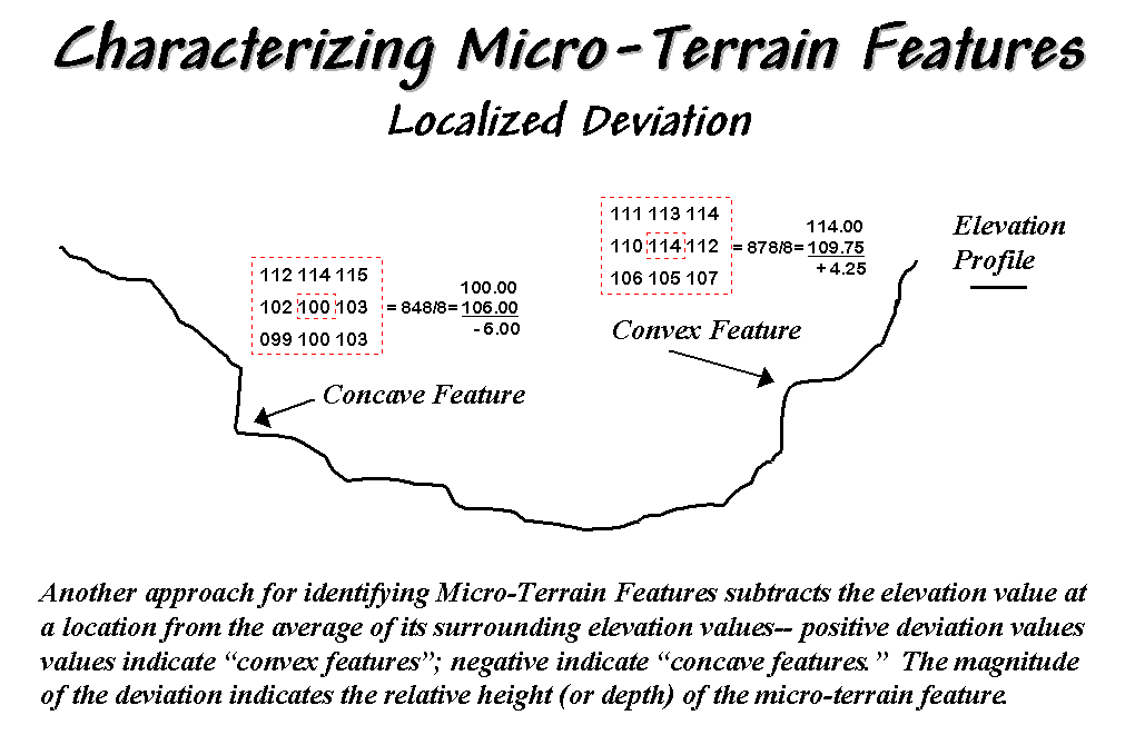 Figure 3. Localized deviation uses a spatial filter to
compare a location to its surroundings.
Figure 3. Localized deviation uses a spatial filter to
compare a location to its surroundings.
The
localized deviation within a roving window is calculated by
subtracting the average of the surrounding elevations from the center
location's elevation. As depicted in
the example calculations for the concave feature, the average elevation of the
surroundings is 106, that results in a -6.00 deviation when subtracted from the
center's value of 100. The negative
sign denotes a concavity while the magnitude of 6 indicates it's fairly
significant dip (a 6/100= .06). The
protrusion above its surroundings (termed a convex feature) shown
on the right of the figure has a localized deviation of +4.25 indicating a
somewhat pronounced bump (4.25/114= .04).
The
result of moving a deviation filter throughout an elevation surface is shown in
the top right inset in figure 4. Its
effect is nearly identical to the trend analysis described before-- comparison
of each location's actual elevation to the typical elevation (trend) in its
vicinity. Interpretation of a Deviation
Surface is the same as that for the difference surface—protrusions (large
positive values) locate drier convex areas; depressions (large negative values)
locate wetter concave areas.
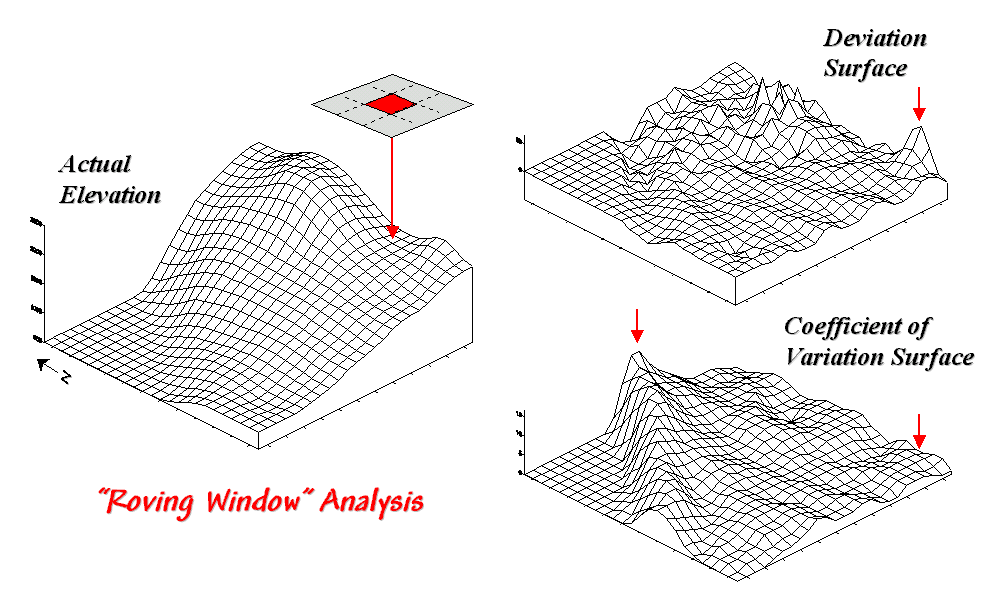 Figure 4. Applying Deviation and Coefficient of
Variation filters to an elevation surface.
Figure 4. Applying Deviation and Coefficient of
Variation filters to an elevation surface.
The
implication of the "Localized Deviation" approach goes far beyond
simply an alternative procedure for calculating terrain irregularities. The use of "roving windows"
provides a host of new metrics and map surfaces for assessing micro-terrain characteristics. For example, consider the Coefficient
of Variation (Coffvar) Surface shown in the bottom-right portion of
figure 4. In this instance, the
standard deviation of the window is compared to its average elevation—small
"coffvar" values indicate areas with minimal differences in
elevation; large values indicate areas with lots of different elevations. The large ridge in the coffvar surface in
the figure occurs along the shoreline of a lake. Note that the ridge is largest for the steeply-rising terrain
with big changes in elevation. The
other bumps of surface variability noted in the figure indicate areas of less
terrain variation.
While
a statistical summary of elevation values is useful as a general indicator of
surface variation or "roughness," it doesn't consider the pattern of the
differences. A checkerboard pattern of
alternating higher and lower values (very rough) cannot be distinguished from
one in which all of the higher values are in one portion of the window and
lower values in another.
There
are several roving window operations that track the spatial arrangement of the
elevation values as well as aggregate statistics. A frequently used one is terrain slope that calculates the
"slant" of a surface. In
mathematical terms, slope equals the difference in elevation (termed the
"rise") divided by the horizontal distance (termed the
"run").
As
shown in figure 5, there are eight surrounding elevation values in a 3x3 roving
window. An individual slope from the
center cell can be calculated for each one.
For example, the percent slope to the north (top of the window) is
((2332 - 2262) / 328) * 100 = 21.3%.
The numerator computes the rise while the denominator of 328 feet is the
distance between the centers of the two cells.
The calculations for the northeast slope is ((2420 - 2262) / 464) * 100
= 34.1%, where the run is increased to account for the diagonal distance (328 *
1.414 = 464).
The
eight slope values can be used to identify the Maximum, the Minimum and the
Average slope as reported in the figure.
Note that the large difference between the maximum and minimum slope (53
- 7 = 46) suggests that the overall slope is fairly variable. Also note that the sign of the slope value
indicates the direction of surface flow—positive slopes indicate flows into the
center cell while negative ones indicate flows out. While the flow into the center cell depends on the uphill
conditions (we'll worry about that in a subsequent section), the flow away from
the cell will take the steepest downhill slope (southwest flow in the example…
you do the math).
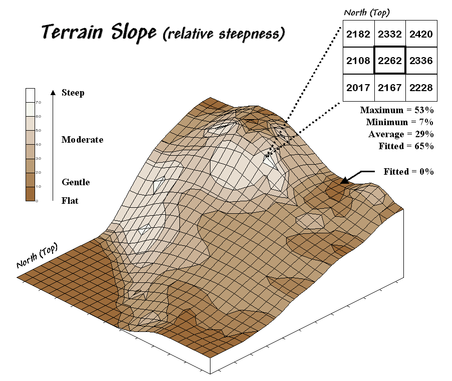 Figure 5. Calculation of slope considers the
arrangement and magnitude of elevation differences within a roving window.
Figure 5. Calculation of slope considers the
arrangement and magnitude of elevation differences within a roving window.
In
practice, the "average slope" can be misleading. It is supposed to indicate the overall slope
within the window but fails to account for the spatial arrangement of the slope
values. An alternative technique
"fits a plane" to the nine individual elevation values. The procedure determines the best fitting
plane by minimizing the deviations from the plane to the elevation values. In the example, the Fitted slope is 65%…
more than the maximum individual slope.
At first this might seem a bit fishy—overall slope more than the maximum
slope—but believe me, determination of fitted slope is a different kettle of fish
than simply scrutinizing the individual slopes.
Numerical
Analysis and Surface Modeling
The
previous sections have presented several techniques for generating maps that
identify the bumps (convex features), the dips (concave features)
and the tilt (slope) of a terrain surface. Although the procedures have a wealth of practical applications,
the underlying hidden agenda of the discussion is to get you thinking of
geographic space in a less traditional way—as an organized set of numbers (numerical
data), instead of points, lines and areas represented by various colors and
patterns (graphic map features).
A
terrain surface is organized as a rectangular "analysis grid" with
each cell containing an elevation value.
Grid-based processing involves retrieving values from one or more of
these "input data layers" and performing a mathematical or
statistical operation on the subset of data to produce a new set numbers. While computer mapping or spatial
database management often operates with the numbers defining a map,
these types of processing simply repackage the existing information. A spatial query to "identify all the
locations above 8000' elevation in El Dorado County" is a good example
of a repackaging interrogation.
Map
analysis
operations, on the other hand, create entirely new spatial information. For example, a map of terrain slope can be
derived from an elevation surface, then used to expand the geo-query to "identify
all the locations above 8000' elevation in El Dorado County (existing data)
that exceed 30% slope (derived data)." While the discussion in this series of columns focuses on
applications in terrain analysis, the subliminal message is much broader—map
analysis procedures derive new spatial information from existing information.
Further
Consideration of Slope
Now
back to the business of characterizing map surfaces. The previous discussions described several approaches for
calculating terrain slope from an elevation surface. Each of the approaches used a "3x3 roving window" to
retrieve a subset of data, yet applied a different analysis function (maximum,
minimum, average or "fitted" summary of the data).
Figure
6 shows the slope map derived by "fitting a plane" to the nine
elevation values surrounding each map location. The inset in the upper left corner of the figure shows a 2-D
display of the slope map. Note that
steeper locations primarily occur in the upper central portion of the area,
while gentle slopes are concentrated along the left side.
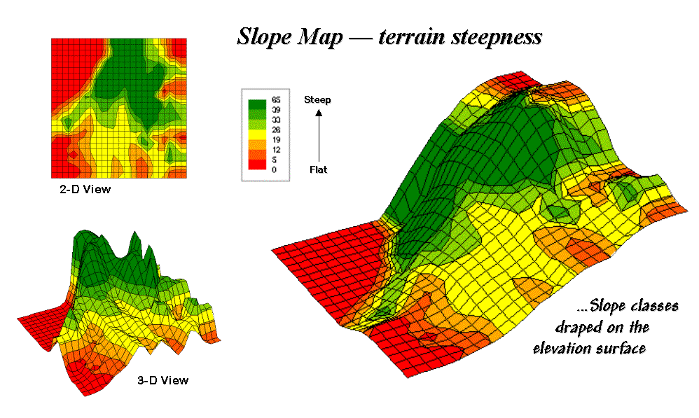 Figure 6. 2-D, 3-D and draped
displays of terrain slope.
Figure 6. 2-D, 3-D and draped
displays of terrain slope.
The
inset on the right shows the elevation data as a wire-frame plot with the slope
map draped over the surface. Note the
alignment of the slope classes with the surface configuration—flat slopes where
it looks flat; steep slopes where it looks steep.
The
3-D view of slope in the lower left, however, looks a bit strange. The big bumps on this surface identify steep
areas with large slope values. The
ups-and-downs (undulations) are particularly interesting. If the area was perfectly flat, the slope
value would be zero everywhere and the 3-D view would be flat as well. But what do you think the 3-D view would
look like if the surface formed a steeply sloping plane?
Are
you sure? The slope values at each location
would be the same, say 65% slope, therefore the 3-D view would be a flat plane
"floating" at a height of 65.
That suggests a useful principle—as a slope map progresses from a
constant plane (single value everywhere) to more ups-and-downs (bunches of
different values), an increase in terrain roughness is indicated.
 Figure 7. Assessing terrain roughness through the 2nd
derivative of an elevation surface.
Figure 7. Assessing terrain roughness through the 2nd
derivative of an elevation surface.
Figure
7 outlines this concept by diagramming the profiles of three different terrain
cross-sections. An elevation surface's
2nd derivative (slope of a slope map) quantifies the amount of
ups-and-downs of the terrain. For the
straight line on the left, the "rate of change in elevation per unit
distance" is constant with the same difference in elevation everywhere
along the line—slope = 65% everywhere.
The resultant slope map would have the value 65 stored at each grid
cell, therefore the "rate of change in slope" is zero everywhere
along the line (no change in slope)—slope2 = 0% everywhere.
A
slope2 value of zero is interpreted as a perfectly smooth condition, which in
this case happens to be steep. The
other profiles on the right have varying slopes along the line, therefore the
"rate of change in slope" will produce increasing larger slope2
values as the differences in slope become increasingly larger.
So
who cares? Water drops for one, as
steep smooth areas are ideal for downhill racing, while "steep 'n rough
terrain" encourages more infiltration, with "gentle yet rough
terrain" the most.
Figure
8 shows a roughness map based on the 2nd derivative for the same
terrain as depicted in Figure 6. Note
the relationships between the two figures.
The areas with the most "ups-and-downs" on the slope map in
figure 6 correspond to the areas of highest values on the roughness map in
figure 8.
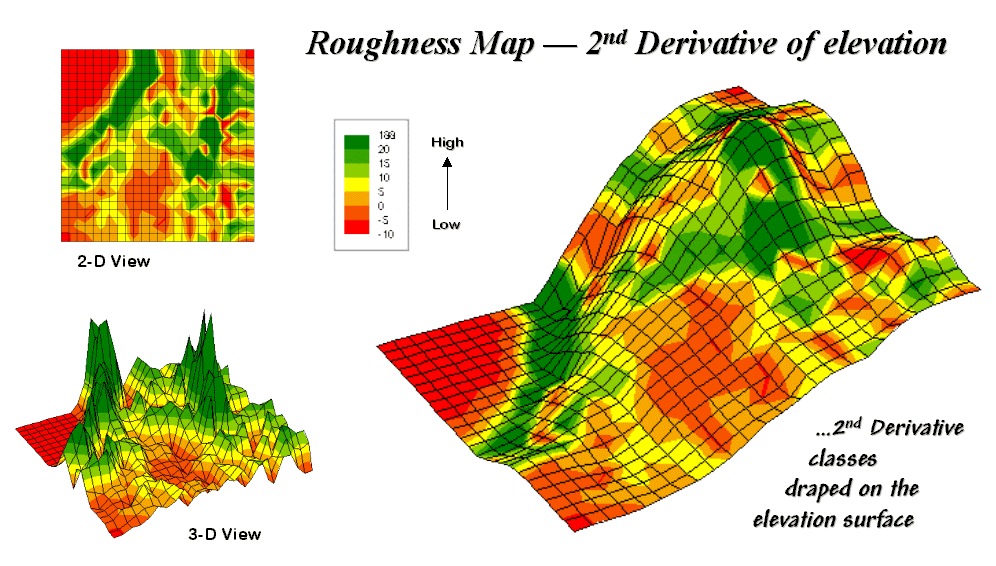 Figure 8. 2-D, 3-D and draped displays of terrain roughness.
Now
focus your attention on the large steep area in the upper central portion of
the map. Note the roughness differences
for the same area as indicated in figure 8—the favorite raindrop racing areas
are the smooth portions of the steep terrain occurring along the central
portion of the front face of the hill.
Mapping
Water Confluence
The
preceding section focused on terrain steepness and roughness. While the concepts are simple and
straightforward, the mechanics of computing them are a bit more
challenging. As you hike in the
mountains your legs sense the steepness and your mind is constantly assessing
terrain roughness. A smooth, steeply-sloped
area would have you clinging to things while a rough steeply-sloped area would
look more like stair steps.
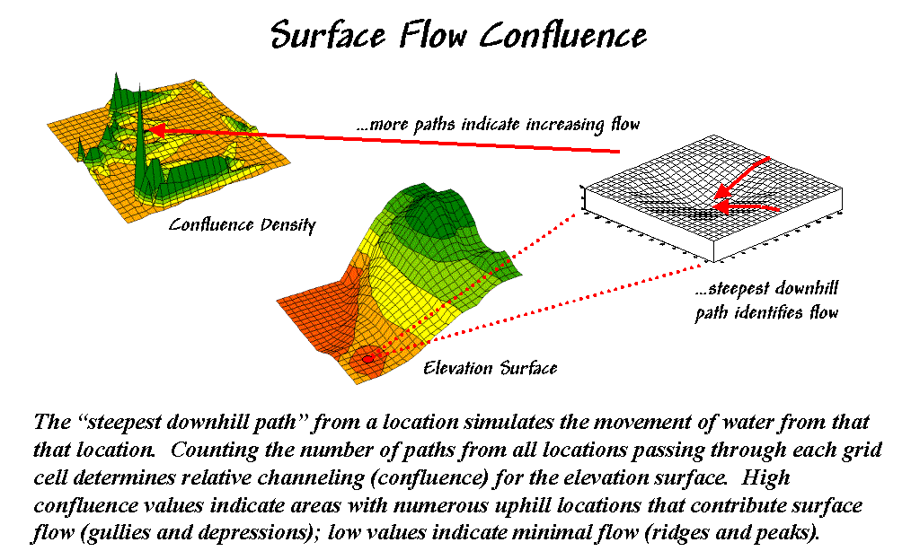 Figure 9. Map of surface flow confluence.
Water
has a similar vantage point of the slopes it encounters, except given its head,
water will take the steepest downhill path, sort of like an out-of-control
skier. Figure 9 shows a map of surface
flow confluence. It is based on the
assumption that water will follow a path that chooses the steepest downhill
step at each point (grid cell) along the terrain surface. In effect, a drop of water is placed at each
location and allowed to pick its path down the terrain surface. Each grid cell that is traversed gets the
value one added to it. As the paths
from other locations are considered the areas sharing common paths get
increasing larger values.
The
inset on the right shows the path taken by a couple of drops into a slight
depression. The inset on the left shows
the considerable inflow for the depression as a high peak in the 3-D display. The high value indicates that a lot of
uphill locations are connected to this feature. However, note that the pathways to the depression are
concentrated along the southern edge of the area.
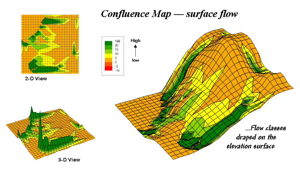 Figure 10. 2-D, 3-D and draped displays of surface flow
confluence.
Figure 10. 2-D, 3-D and draped displays of surface flow
confluence.
Ridges
on the confluence density surface identify areas of high surface flow. In figure 10, note how these areas (darker)
align with the creases in the terrain as shown on the draped elevation surface
on the right. The 2-D map provides a
more familiar map rendering of where not to unroll your sleeping bag if flash
floods are likely.
Putting
It All Together
The
various spatial analysis techniques for characterizing terrain surfaces provide
a wealth of different perspectives on surface configuration. Deviation from Trend, Difference
Maps and Deviation Surfaces are used to identify areas that
"bump-up" (convex) or "dip-down" (concave). A Coefficient of Variation Surface looks
at the overall disparity in elevation values occurring within a small
area. A Slope Map shares a
similar algorithm (roving window) but the summary of is different and reports
the "tilt" of the surface. An
Aspect Map extends the analysis to include the direction of the tilt as
well as the magnitude. The Slope of
a Slope Map (2nd derivative) summarizes the frequency of the
changes along an incline and reports the roughness throughout an elevation
surface. Finally, a Confluence Map
takes an extended view and characterizes the number of uphill locations
connected to each location.
The
coincidence of these varied perspectives can provide valuable input to
decision-making. Areas that are smooth,
steep and coincide with high confluence are strong candidates for gully-washers
that gouge the landscape. On the other
hand, areas that are rough, gently-sloped and with minimal confluence are
relatively stable. Concave features in
these areas tend to trap water and recharge soil moisture and the water table. Convex features under erosive conditions
tend to become more prominent as the confluence of water flows around it.
Similar
interpretations can be made for hikers, who like raindrops react to surface
configuration in interesting ways.
While steep, smooth surfaces are avoided by all but the rock-climber,
too gentle surfaces tend too provide boring hikes. Prominent convex features can make interesting areas for
viewing—from the top for hearty and from the bottom for the aesthetically
bent. Areas of water confluence don't
mix with hiking trail unless a considerable number of water-bars are placed in
the trail.
While
these "rules-of-thumb" make sense in a lot of circumstances, there
are numerous exceptions that undercut them.
Two concerns are particularly important. First, conditions along the surface can alter the effect of
terrain characteristics. For example,
soil properties and vegetation present greatly effect surface runoff and
sediment transport. The nature of
accumulated distance along the surface
In
addition, the resolution of the elevation grid can effect the
calculations. In the case of water
drops the gridding resolution must be high to capture the subtle twists and
bends that direct water flow. A hiker
on the other hand, is less sensitive to subtle changes in elevation. The rub is that collection of the
appropriate elevation is prohibitive in most practical applications. The result is that existing elevation data,
such as the USGS Digital Terrain Models (DTM), are used in most cases. Since the GIS procedures are independent of
the gridding resolution, inappropriate maps can be generated and used in
decision-making. The recognition of the
importance of spatial analysis and surface modeling is imperative. Its effective use requires informed and wary
users.
_____________________________________
Author's
Note: This paper is based on a series
of "Beyond Mapping" columns on characterizing micro-terrain appearing
in GeoWorld magazine, January through April, 2000. The calculations and displays using MAPcalc software by Red Hen
Systems, Inc., 2310 East Prospect Road, Suit A, Fort Collins, USA 80525, (800)
237-4182, Email: info@redhensystems.com,
Web site: http://www.redhensystems.com/
1 Joseph K.
Berry is President of Berry & Associates // Spatial Information Systems,
Inc., consultants and software developers in GIS technology.