…the following is from a
three-part series on Landscape Rendering appearing in the “Beyond Mapping”
column by
______________________
Behind the Scenes of Virtual Reality (GEOWorld online June, 2000)
Over the past three decades,
cutting-edge GIS has evolved from computer mapping to spatial
database management, and more recently, to map analysis and modeling. The era of a sequestered GIS specialist has
given way to mass marketed applications, such as MapQuest’s geo-queries,
On-Star’s vehicular telematics and a multitude of other Internet-served maps.
The transition of GIS from an
emerging industry to a fabric of society has radically changed traditional
perspectives of map form, content and applications. Like a butterfly emerging from a cocoon,
contemporary maps are almost indistinguishable from their predecessors. While underlying geographic principles
remain intact, outward appearances of modern maps are dramatically different.
This evolution is most
apparent in multimedia GIS.
Traditional maps graphically portray map features and conditions as
static, 2-D abstractions composed of pastel colors, shadings, line types and
symbols. Modern maps, on the other hand,
drapes spatial information on 3-D surfaces and provides interactive query of
the mapped data that underlies the pictorial expression. Draped remote sensing imagery enables a user
to pan, zoom and rotate the encapsulated a picture of actual conditions. Map features can be hyperlinked to text,
tables, charts, audio, still images and even streaming video. Time series data can be sequenced to animate
changes and enhance movement of in both time and space.
While these visualizations
are dramatic, none of the multimedia GIS procedures shake the cartographic
heritage of mapping as much as virtual reality. This topic was introduced in a feature
article in GeoWorld a few years ago (Visualize Realistic Landscapes, GeoWorld,
August, 1998, pages 42-47). This and the
next couple of columns will go behind the scenes to better understand how 3-D
renderings are constructed and investigate some of the approaches important
considerations and impacts.
Since discovery of herbal
dyes, the color pallet has been a dominant part of mapping. A traditional map of forest types, for
example, associates various colors with different tree species—red for
ponderosa pine, blue for Douglas fir, etc.
Cross-hatching or other cartographic techniques can be used to indicate
the relative density of trees within each forest polygon. A map’s legend relates the abstract colors and
symbols to a set of labels identifying the inventoried conditions. Both the map and the text description are
designed to conjure up a vision of actual conditions and the resulting spatial
patterns.
The map has long served as an
abstract summary while the landscape artist’s canvas has served as a more
realistic rendering of a scene. With the
advent of computer maps and virtual reality techniques the two perspectives are
merging. In short, color pallets
are being replaced by rendering pallets.
Like the artist’s painting,
complete objects are grouped into patterns rather than a homogenous color
applied to large areas. Object types,
size and density reflect actual conditions.
A sense of depth is induced by plotting the objects in perspective. In effect, a virtual reality GIS “sees” the
actual conditions of forest parcels through its forest inventory data— species
type, mixture, age, height and stocking density for each parcel. A composite scene is formed by translating
the data into realistic objects that characterize trees, houses, roads and
other features then combined with suitable textures to typify sky, clouds,
soil, brush and grasses.
Fundamental to the process is
the ability to design realistic objects.
An effective approach, termed geometric modeling, utilizes an
interface (figure 1) similar to a 3-D computer-aided drafting system to
construct individual scene elements. A
series of sliders and buttons are used to set the size, shape, orientation and
color of each element comprising an object.
For example, a tree is built by specifying a series of levels
representing the trunk, branches, and leaves.
Level one forms the trunk that is interactively sized until the designer
is satisfied with the representation.
Level two establishes the pattern of the major branches. Subsequent levels identify secondary
branching and eventually the leaves themselves.
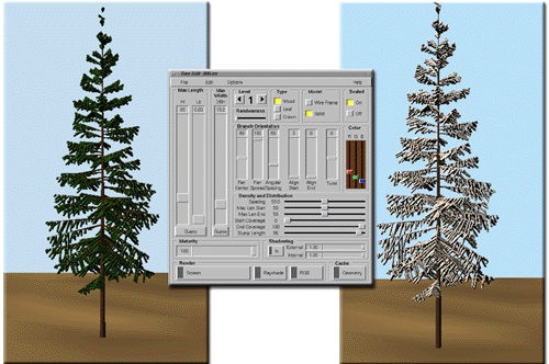 Figure 1. Designing tree objects.
The basic factors that define
each level include 1) linear positioning, 2) angular positioning, 3)
orientation, 4) sizing and 5) representation.
Linear positioning determines how often and where branches
occur. In fig. 1, the major branching
occurs part way up the trunk and is fairly evenly spaced.
The angular positioning,
sets how often branches occur around the trunk or branch to which it is
attached. The branches at the third
level in the figure form a fan instead of being equally distributed around the
branch. Orientation refers to how
the branches are tilting. Note that the
lower branches droop down from the trunk, while the top branches are more
skyward looking. The third-order
branches tend show a similar drooping effect in the lower branches.
Sizing defines the length and taper a particular
branch. In the figure, the lower
branches are considerably smaller than the mid-level branches. Representation covers a lot of factors
identifying how a branch will appear when it is displayed, such as its
composition (a stick, leaf or textured crown), degree of randomness, and 24-bit
RGB color. In figure 1, needle color and
shading was changed for the tree on the right to simulate a light dusting of
snow. Other effects such as fall
coloration, leaf-off for deciduous trees, disease dieback, or pest infestations
can be simulated.
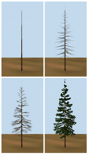
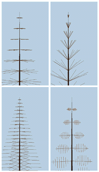 Figure 2. The inset on the left shows various branching
patterns. The inset on the right depicts
the sequencing of four branching levels.
Figure 2. The inset on the left shows various branching
patterns. The inset on the right depicts
the sequencing of four branching levels.
Figure 2 illustrates some
branching patterns and levels used to construct tree-objects. The tree designer interface at first might
seem like overkill—sort of a glorified “painting by the numbers.” While it’s useful for the
artistically-challenged, it is critical for effective 3-D rendering of virtual
landscapes.
The mathematical expression
of an object allows the computer to generate a series of “digital photographs” of
a representative tree under a variety of look-angles and sun-lighting
conditions. The effect is similar to
flying around the tree in a helicopter and taking pictures from different
perspectives as the sun moves across the sky.
The background of each bitmap is made transparent and the set is added
to the library of trees. The result is a
bunch of snapshots that are used to display a host of trees, bushes and shrubs
under different viewing conditions.
The object-rendering
process results in a “palette” of objects analogous to the color palette
used in conventional GIS systems. When
displaying a map, the GIS relates a palette number with information about a
forest parcel stored in a database. In
the case of 3-D rendering, however, the palette is composed of a multitude of
tree-objects. The effect is like
color-filling polygons, except realistic trees are poured onto the landscape
based on the tree types, sizing and densities stored in the GIS. How this scene rendering process works is
reserved for next month.
_______________________
Author's Note: the Tree
designer module of the Virtual Forest software package by Pacific Meridian
Resources was used for the figures in this column. See http://www.innovativegis.com/products/vforest/
for more examples and discussion.
Constructing a Virtual Scene (GEOWorld online July, 2000)
The previous column described
how 3-dimensional objects, such as trees, are built for use in generating
realistic landscape renderings. The
drafting process uses an interface that enables a user to interactively adjust
the trunk’s size and shape then add branches and leaves with various angles and
positioning. The graphic result is
similar to an artist’s rendering of an individual tree.
The digital representation,
however, is radically different. Because
it is a mathematically defined object, the computer can generate a series of
“digital photographs” of the tree under a variety of look-angles and
sun-lighting conditions. The effect is
similar to flying around the tree in a helicopter and taking pictures from
different perspectives as the sun moves across the sky.
The background of each of
these snapshots is made transparent and the set is added to a vast library of
tree symbols. The result is a set of
pictures that are used to display a host of trees, bushes and shrubs under
different viewing conditions. A virtual
reality scene of a landscape is constructed by pasting thousands of these
objects in accordance with forest inventory data stored in a GIS.
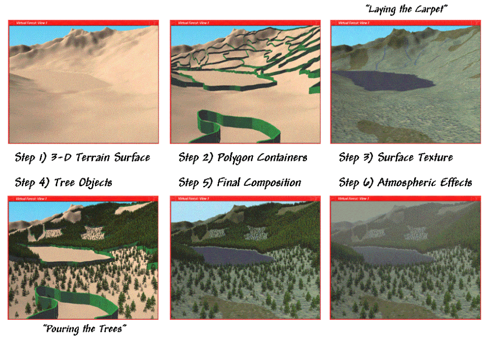
Figure 1. Basic steps in constructing a virtual reality
scene.
There are six steps in
constructing a fully rendered scene (see Figure 1). A digital terrain surface provides the lay of
the landscape. The GIS establishes the
forest stand boundaries as geo-registered polygons with attribute data
describing stand make-up and condition.
The link between the GIS data
and the graphic software is critical.
For each polygon, the data identifies the types of trees present, their
relative occurrence (termed stocking density) and maturity (age, height). In a mixed stand, such as spruce, fir and
interspersed aspen, several tree symbols will be used. Tree stocking identifies the number of trees per
acre for each of the species present.
This information is used to determine the number tree objects to “plant”
and cross-link to the appropriate tree symbols in 3-D tree object library. The relative positioning of the polygon on
the terrain surface with respect to the viewpoint determines which snapshot of
the tree provides the best view and sun angle representation.
Finally, information on
percent maturity establishes the baseline height of the tree. In a detailed tree library several different
tree objects are generated to represent the continuum from immature, mature and
old growth forms. Figure 2 shows the
tree exam files for two polygons identified in the adjacent graphic. The first column of values identifies the
tree symbol (library ID#). Polygon 1573
has 21 distinct tree types including snags (dead trees). Polygon 1658 is much smaller and only
contains 16 different types. The second
column indicates the percent maturity while the third defines the number of
trees. These data shown are for an
extremely detailed U.S. Forest Service research area in
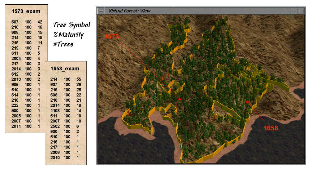 Figure 2. Forest inventory data establishes tree types,
stocking density and maturity.
Figure 2. Forest inventory data establishes tree types,
stocking density and maturity.
Once the appropriate tree symbol
and number of trees are identified the computer can begin “planting” them. This step involves determining a specific
location within the polygon and sizing the snapshot based on the tree’s
distance from the viewpoint. Most often
trees are randomly placed however clumping and compaction factors can be used
to create clustered patterns if appropriate.
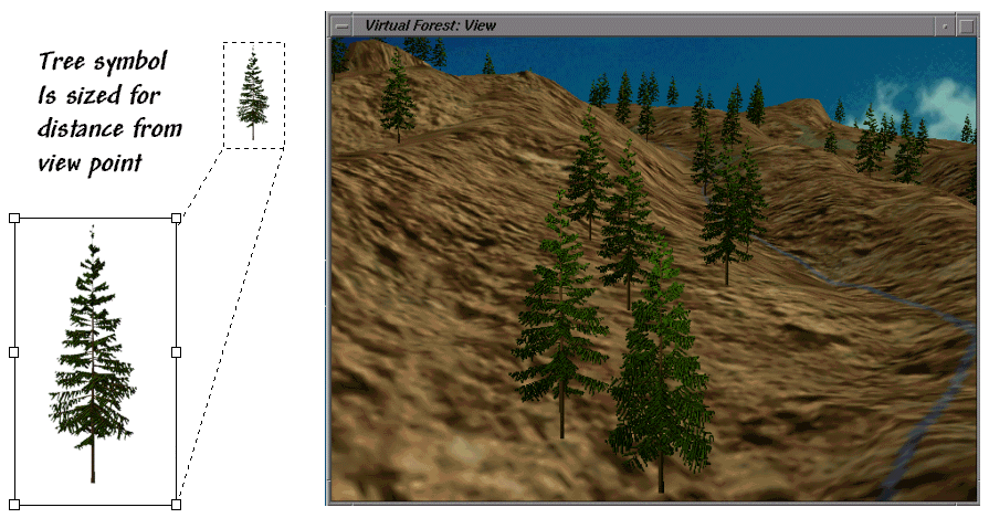 Figure 3. Tree symbols are “planted” then sized
depending on their distance from the viewpoint.
Figure 3. Tree symbols are “planted” then sized
depending on their distance from the viewpoint.
Tree sizing is similar
pasting and resizing an image in a word document. The base of the tree symbol is positioned at
the specific location then enlarged or reduced depending on how far the tree is
from the viewing position. Figure 3
shows a series of resized tree symbols “planted” along a slope—big trees in
front and progressively smaller ones in the distance.
The process of rendering a
scene is surprisingly similar to that of landscape artist. The terrain is painted and landscape features
added. In the artist’s world it can take
hours or days to paint a scene. In
virtual reality the process is completed in a minute or two as hundreds of trees
are selected, positioned and resized each second.
Since each tree is embedded
on a transparent canvas they obscure what is behind them—textured terrain
and/or other trees, depending on forest stand and viewing conditions. Terrain locations that are outside of the
viewing window or hidden behind ridges are simply ignored. The multitude of issues and extended
considerations surrounding virtual reality’s expression of GIS data, however,
cannot be ignored. That discussion is
reserved for next month.
_______________________
Author's Note: the
Landscape Viewer module of the Virtual Forest software package by Pacific
Meridian Resources was used for the figures in this column. See http://www.innovativegis.com/products/vforest/
for more examples and discussion.
Representing Changes in a Virtual Forest
Previous columns (GEOWorld,
?? and ??) described the steps in rendering a virtual landscape. The process begins with a 3D drafting program
used to construct mathematical representations of individual scene elements
similar to a painter’s sketches of the different tree types that occur within
an area. The tree library is linked to
GIS data describing the composition of each forest parcel. These data are used to position the polygon
on the terrain, select the proper understory texture (“laying the carpet”)
and paste the appropriate types and number of trees within each polygon (“pouring
the trees”).
The result is a strikingly
lifelike rendering of the landscape instead of a traditional map. While maps use colors and abstract symbols to
represent forest conditions, the virtual forest uses realistic scene elements
to reproduce the composition and structure of the forest inventory data. This lifelike 3D characterization of spatial
conditions extends the boundaries of mapping from dry and often confusing
drawings to more familiar graphical perspectives.
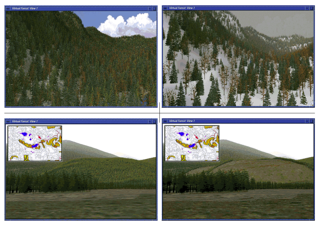 Figure 1. Changes in the landscape can be visualized by
modifying the forest inventory data.
Figure 1. Changes in the landscape can be visualized by
modifying the forest inventory data.
The baseline rendering for a
data set can be modified to reflect changes on the landscape. For example, the top two inserts in figure 1
depict a natural thinning and succession after a severe insect infestation. The winter effects were introduced by
rendering with a snow texture and an atmospheric haze.
The lower pair of inserts
show the before and after views of a proposed harvest block. Note the linear texture features in the
clearcut that identify the logging road.
Alternative harvest plans can be rendered and their relative visual
impact assessed. In addition, a temporal
sequence can be generated that tracks the ‘green-up” through forest growth
models as a replanted parcel grows. In a
sense, the baseline GIS information shows you “what is,” while the rendering of
the output from a simulation model shows you “what could be.”
While GIS modeling can walk
through time, movement to different viewpoints provides a walk through the
landscape. The viewer position can be
easily changed to generate views from a set of locations, such as sensitive
viewpoints along a road or trail. Figure
2 shows the construction of a ‘fly-by” movie.
The helicopter flight path at 200 meters above the terrain was digitized
then resampled every twenty meters (large red dots in the figure). A full 3D rendering was made for each of the
viewpoints (nearly 900 in all) and, when viewed at 30 frames per second, forms
a twenty-eight second flight through the GIS database (see author’s note).
Admittedly, real-time
“fly-bys” of GIS databases are a bit futuristic. With each scene requiring three to four
minutes to fully render on a PC-level computer, a 30 second movie requires
about 45 hours of processing time. The
Lucas Films machines would reduce the time to a few minutes but it will take a
few years to get that processing power on most desktops. In the interim, the transition from
traditional maps to fully rendered scenes is operationally constrained to a few
vanguard software systems.
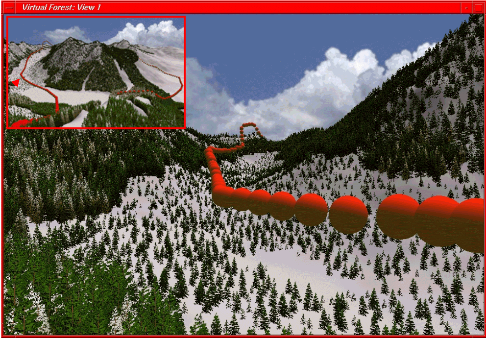 Figure 2. A “fly-by” movie is constructed by generating
a sequence of renderings then viewing them in rapid succession.
Figure 2. A “fly-by” movie is constructed by generating
a sequence of renderings then viewing them in rapid succession.
There are several concerns
about converting GIS data into realistic landscape renderings. Tree placement is critical. Recall that “stocking” (#trees per acre) is
the forest inventory statistic used to determine the number of trees to paste
within a polygon. While this value
indicates the overall density it assumes the trees are randomly distributed in
geographic space.
While trees off in the
distance form a modeled texture, placement differences of a couple of feet for
trees in the foreground can significantly alter a scene. For key viewpoints GPS positioning of
specific trees within a few feet of the viewer is required. Also, in sequential rendering the trees are
statistically placed for the first scene then that “tree map” is used for all
of the additional scenes. Many species,
such as aspen, tend to group and statistical methods are needed to account for
“clumping” (number of seed trees) and “compaction” (distance
function from seed tree).
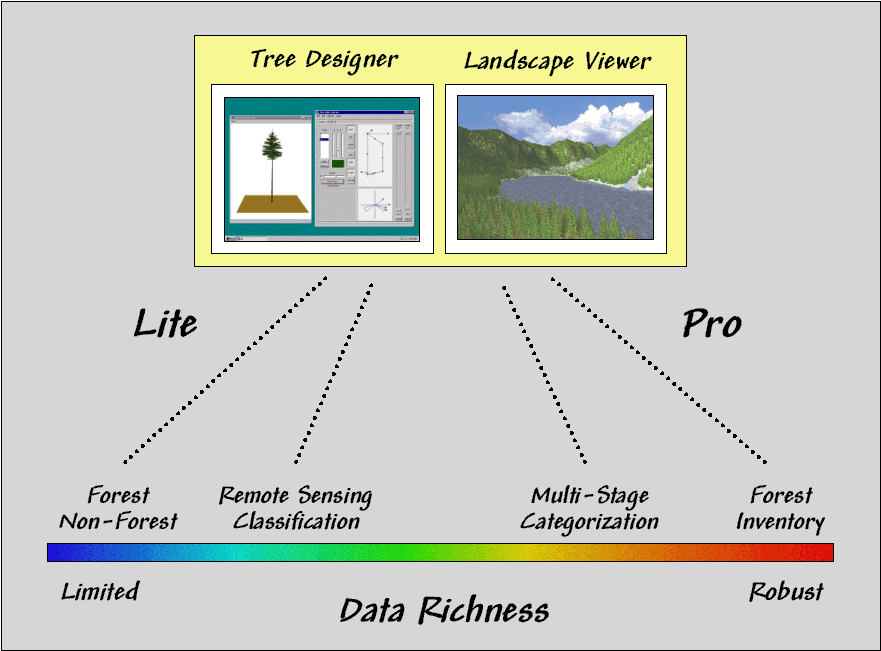 Figure 3. Strikingly real snapshots of forest data can
be generated from either limited or robust GIS data.
Figure 3. Strikingly real snapshots of forest data can
be generated from either limited or robust GIS data.
Realistic trees, proper
placement, appropriate understory textures and shaded relief combine to produce
strikingly real snapshots of a landscape.
In robust, forest inventory data the rendering closely matches reality. However, equally striking results can be
generated from limited data. For
example, the “green” portions on topographic maps indicate forested areas, but
offer no information about species mixture, age/maturity or stocking. Within a GIS, a “best guess” (er… expert
opinion) can be substituted for the field data and one would be hard-pressed to
tell the differences in rendered scenes.
That brings up an important
point as map display evolves to virtual reality—how accurate is the
portrayal? Our cartographic legacy has
wrestled with spatial and thematic accuracy, but “rendering fidelity” is
an entirely new concept. Since you can’t
tell by looking, standards must be developed and integrated with the metadata
accompanying a rendering. Interactive
links between the underlying data and the snapshot are needed. Without these safeguards, it’s “viewer
beware” and opens a whole new avenue for lying with maps.
While Michael Creighton’s
emersion into a virtual representation of a database (the novel Disclosure)
might be decades off, virtual renderings of GIS data is a quantum leap
forward. The pastel colors and abstract
symbols of traditional maps are becoming endangered cartographic
procedures. When your grandchild conjures
up a 3D landscape with real-time navigation on a wrist-PC, you’ll fondly recall
the bumpy transition from our paper-map paradigm.
_______________________
Author's Note: the
Virtual Forest software package by Pacific Meridian Resources was used for the
figures in this column. See http://www.innovativegis.com/products/vforest/,
select “Flybys” to access the simulated helicopter flight described as well as
numerous other examples of 3D rendering.