Beyond
Mapping III
|
Map
Analysis book with companion CD-ROM
for hands-on exercises and further reading |
Use
Data to Characterize Micro-Terrain Features — describes
techniques to identify convex and concave features
Characterizing
Local Terrain Conditions — discusses
the use of "roving windows" to distinguish localized variations
Characterizing
Terrain Slope and Roughness — discusses
techniques for determining terrain inclination and coarseness
The Long and Short of Slope
— investigates
longitudinal and transverse slope calculation
Generating
Mountains and Molehills from Field Sampled Data — creating
an elevation surface from field sampled data
Segmenting Our World — discusses
techniques for segmenting linear routes based on terrain inflection
Confluence Maps Further Characterize Micro-terrain
Features —
describes the use of optimal path density analysis for mapping surface flows
Modeling Erosion and
Sediment Loading — illustrates
a
Identify Valley Bottoms in Mountainous Terrain
— illustrates a
technique for identifying flat areas connected to streams
Use Surface Area for Realistic Calculations
— describes a
technique for adjusting planimetric area to surface area considering terrain
slope
Beware of Slope’s Slippery Slope
— describes
various slope calculations and compares results
Shedding Light on Terrain Analysis — discusses how terrain orientation is used to generate Hillshade maps
Identifying Upland Ridges — describes a procedure for locating extended upland ridges
Note: The processing and figures discussed in this topic were derived using MapCalcTM
software. See www.innovativegis.com to download a
free MapCalc Learner version with tutorial materials for classroom and
self-learning map analysis concepts and procedures.
<Click here>
right-click to download a
printer-friendly version of this topic (.pdf).
(Back to the Table of
Contents)
______________________________
Use Data
to Characterize Micro-Terrain Features
(GeoWorld January, 2000; “” pg.
22)
The past several columns investigated surface modeling and
analysis. The data surfaces derived in
these instances weren't the familiar terrain surfaces you walk the dog, bike
and hike on. None-the-less they form
surfaces that contain all of the recognizable gullies, hummocks, peaks and
depressions we see on most hillsides.
The "wrinkled-carpet" look in the real world is directly
transferable to the cognitive realm of the data world.
Figure 31-1. Identifying
Convex and Concave features by deviation from the trend of the terrain.
One of the most
frequently used procedures involves comparing the trend of the surface to the
actual elevation values. Figure 31-1
shows a terrain profile extending across a small gully. The dotted line identifies a smoothed curve
fitted to the data, similar to a draftsman's alignment of a French curve. It "splits-the-difference" in the
succession of elevation values—half above and half below. Locations above the trend line identify
convex features while locations below identify the concave ones. The further above or below determines how pronounced
the feature is.
In a
In generating the smoothed surface, elevation values were averaged for a 4-by-4
window moved throughout the area. Note
the subtle differences between the surfaces—the tendency to pull-down the
hilltops and push-up the gullies.
While you see (imagine?) these differences in the surfaces, the computer
quantifies them by subtracting. The
difference surface on the right contains values from -84 (prominent concave
feature) to +94 (prominent convex feature).
The big bump on the difference surface corresponds to the smaller
hilltop on elevation surface. Its actual
elevation is 2016 while the smoothed elevation is 1922 resulting in 2016 - 1922
= +94 difference. In micro-terrain
terms, these areas are likely drier than their surroundings as water flows
away.
The other arrows on the surface indicate other interesting locations. The "pockmark" in the foreground is
a small depression (764 - 796 = -32 difference) that is likely wetter as water
flows into it. The "deep cut"
at the opposite end of the difference surface (539 - 623 = -84) suggests a
prominent concavity. However
representing the water body as fixed elevation isn't a true account of terra
firma configuration and misrepresents the true micro-terrain pattern.
Figure 31-2. Example of a micro-terrain
deviation surface.
In fact the entire
concave feature in the upper left portion of 2-D representation of the difference
surface is suspect due to its treatment of the water body as a constant
elevation value. While a fixed value for
water on a topographic map works in traditional mapping contexts it's
insufficient in most analytical applications.
Advanced
The 2-D map of differences identifies areas that are concave (dark red), convex
(light blue) and transition (white portion having only -20 to +20 feet
difference between actual and smoothed elevation values). If it were a map of a farmer's field, the
groupings would likely match a lot of the farmer's recollection of crop
production—more water in the concave areas, less in the convex areas.
A
The idea of variable rate response to spatial conditions has been around for
thousands of years as indigenous peoples adjusted the spacing of holes they
poked in the ground to drop in a seed and a piece of fish. While the mechanical and green revolutions
enable farmers to cultivate much larger areas they do so in part by applying
broad generalizations of micro-terrain and other spatial variables over large
areas. The ability to continuously
adjust management actions to unique spatial conditions on expansive tracks of
land foretells the next revolution.
Investigate the effects of micro-terrain conditions goes
well beyond the farm. For example, the
Universal Soil Loss Equation uses "average" conditions, such as
stream channel length and slope, dominant soil types and existing land use
classes, to predict water runoff and sediment transport from entire
watersheds. These non-spatial models are
routinely used to determine the feasibility of spatial activities, such as
logging, mining, road building and housing development. While the procedures might be applicable to
typical conditions, they less accurately track unusual conditions clumped
throughout an area and provide no spatial guidance within the boundaries of the
modeled area.
Characterizing Localized
Terrain Conditions
(GeoWorld, February 2000, pg. 26)
Last month's column
described a technique for characterizing micro-terrain features involving the
difference between the actual elevation values and those on a smoothed
elevation surface (trend). Positive
values on the difference map indicate areas that "bump-up" while
negative values indicate areas that "dip-down" from the general trend
in the data.
A related technique
to identify the bumps and dips of the terrain involves moving a "roving
window" (termed a spatial filter) throughout an elevation surface. The profile of a gully can have
micro-features that dip below its surroundings (termed concave) as shown on the
right side of figure 31-3.
Figure 31-3. Localized deviation uses a spatial filter to
compare a location to its surroundings.
The localized
deviation within a roving window is calculated by subtracting the average of
the surrounding elevations from the center location's elevation. As depicted in the example calculations for
the concave feature, the average elevation of the surroundings is 106, that computes to a -6.00 deviation when subtracted from the
center's value of 100. The negative sign
denotes a concavity while the magnitude of 6 indicates it's fairly significant
dip (a 6/100= .06). The protrusion above
its surroundings (termed a convex feature) shown on the right of the figure has
a localized deviation of +4.25 indicating a somewhat pronounced bump (4.25/114=
.04).
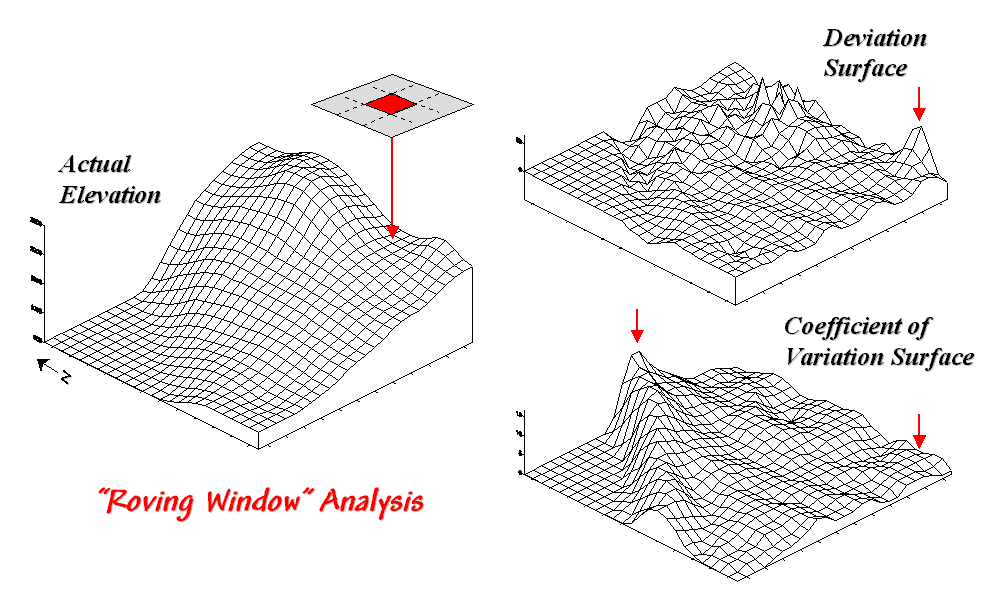
Figure 31-4. Applying Deviation and Coefficient of
Variation filters to an elevation surface.
The result of moving
a deviation filter throughout an elevation surface is shown in the top right
inset in figure 31-4. Its effect is
nearly identical to the trend analysis described last month-- comparison of
each location's actual elevation to the typical elevation (trend) in its
vicinity. Interpretation of a Deviation
Surface is the same as that for the difference surface discussed last
month—protrusions (large positive values) locate drier convex areas;
depressions (large negative values) locate wetter concave areas.
The implication of the "Localized Deviation" approach goes far beyond
simply an alternative procedure for calculating terrain irregularities. The use of "roving windows"
provides a host of new metrics and map surfaces for assessing micro-terrain
characteristics. For example, consider
the Coefficient of Variation (Coffvar) Surface shown
in the bottom-right portion of figure 31-4.
In this instance, the standard deviation of the window is compared to
its average elevation—small "coffvar"
values indicate areas with minimal differences in elevation; large values
indicate areas with lots of different elevations. The large ridge in the coffvar
surface in the figure occurs along the shoreline of a lake. Note that the ridge is largest for the
steeply-rising terrain with big changes in elevation. The other bumps of surface variability noted
in the figure indicate areas of less terrain variation.
While a statistical summary of elevation values is useful as a general
indicator of surface variation or "roughness," it doesn't consider
the pattern of the differences. A
checkerboard pattern of alternating higher and lower values (very rough) cannot
be distinguished from one in which all of the higher values are in one portion
of the window and lower values in another.
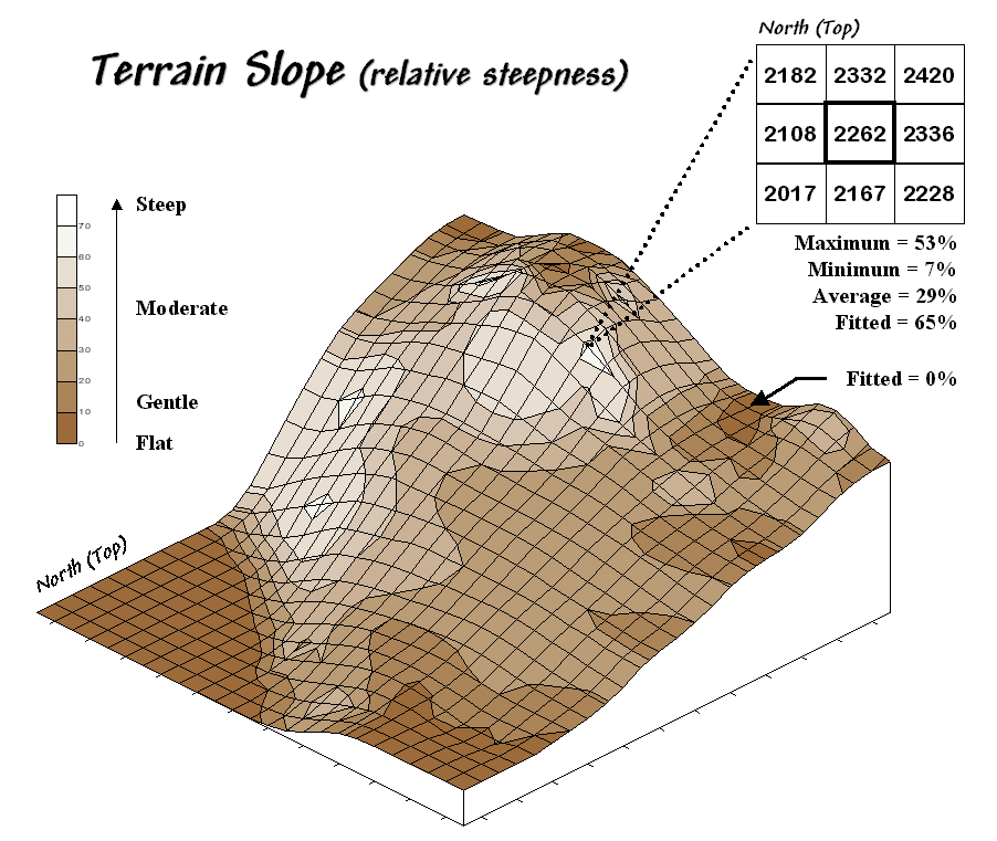
Figure 31-5. Calculation of slope considers the
arrangement and magnitude of elevation differences within a roving window.
There are several
roving window operations that track the spatial arrangement of the elevation
values as well as aggregate statistics.
A frequently used one is terrain slope that calculates the
"slant" of a surface. In
mathematical terms, slope equals the difference in elevation (termed the
"rise") divided by the horizontal distance (termed the
"run").
As shown in figure 31-5, there are eight surrounding elevation values in a 3x3
roving window. An individual slope from
the center cell can be calculated for each one.
For example, the percent slope to the north (top of the window) is
((2332 - 2262) / 328) * 100 = 21.3%. The
numerator computes the rise while the denominator of 328 feet is the distance
between the centers of the two cells.
The calculations for the northeast slope is ((2420 - 2262) / 464) * 100
= 34.1%, where the run is increased to account for the diagonal distance (328 *
1.414 = 464).
The eight slope values can be used to identify the Maximum, the Minimum and the
Average slope as reported in the figure.
Note that the large difference between the maximum and minimum slope (53
- 7 = 46) suggests that the overall slope is fairly variable. Also note that the sign of the slope value
indicates the direction of surface flow—positive slopes indicate flows into the
center cell while negative ones indicate flows out. While the flow into the center cell depends
on the uphill conditions (we'll worry about that in a subsequent column), the
flow away from the cell will take the steepest downhill slope (southwest flow
in the example… you do the math).
In practice, the Average slope can be misleading. It is supposed to indicate the overall slope
within the window but fails to account for the spatial arrangement of the slope
values. An alternative technique fits a
“plane” to the nine individual elevation values. The procedure determines the best fitting
plane by minimizing the deviations from the plane to the elevation values. In the example, the Fitted
slope is 65%… more than the maximum individual slope.
At first this might seem a bit fishy—overall slope more than the maximum
slope—but believe me, determination of fitted slope is a different kettle of
fish than simply scrutinizing the individual slopes. Next time we'll look a bit deeper into this
fitted slope thing and its applications in micro-terrain analysis.
_______________________
Author's Note: An Excel worksheet
investigating Maximum, Minimum, and Average slope calculations is available
online at the "Column Supplements" page at http://www.innovativegis.com/basis.
(GeoWorld, July 2007, pg. 18-19)
Recall from the past sections dealing with slope calculation that the nine elevation values in a 3x3 window are generally used. There are two basic approaches for characterizing relative steepness—surface fitting and individual slope statistics.
Surface fitting aligns a plane to the elevation values that minimizes the deviations from the plane to the values. If all of the values are the same, a horizontal plane is fitted and the slope is zero. However as the values on one side of the window increase and the values on the other decrease, the fitted plane tilts indicating increasing terrain steepness.
The surface fitting algorithm first establishes the 3x3 window, then identifies the nine elevation values, fits the plane and records the slope for the center cell in the window. The “roving window” shifts to the next adjacent location and repeats the process until all of the cells in a project area have been evaluated.
The algorithm for summarizing individual slopes also utilizes a 3x3 window, but instead of fitting a plane it calculates the slopes formed by the center location and each of its eight neighbors. The minimum, maximum or average of the individual slope values is recorded for the center cell and the window advanced.
Both slope techniques result in a continuous map surface indicating the relative steepness throughout a project area. Sometimes, however, slope along a linear feature, such as a pipeline, is sought (figure 1). In this case, only three cells are involved—the center cell and its input and output neighbors at each location along the pipeline.
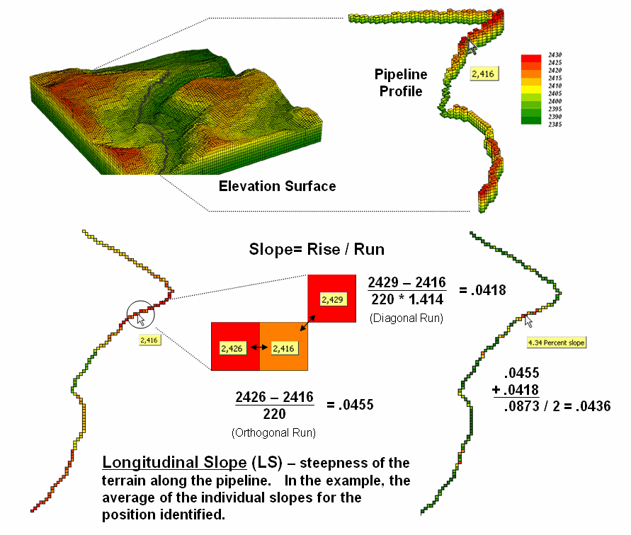
Figure 1. Longitudinal slope calculates the steepness
along a linear feature, such as a pipeline.
Longitudinal Slope (LS) requires isolating just the route’s elevation values. In grid-based modeling this means first creating a “masking map” of the route where the cells defining the pipeline are assigned the value 1 and the non-pipeline cells are assigned a special value of Null (or No Data). This map is multiplied by the elevation surface having the effect of retaining the elevation values along the route but all other locations are assigned Null.
Most map analysis packages have been “trained” to recognize a Null value and simply skip over these locations when processing. The effect in this case is to calculate slope using just the three aligned elevation values in the 3x3 roving window—either fitted or maximum/minimum/average.
A simple extension to the algorithm, Directional Slope (DS), enables a user to enter a starting location and the direction of flow, and then it calculates individual slopes for each step along the route using just the input and center cell. This technique characterizes where gravity is helping or hindering flow and is useful in determining draw-down if the pipe is ruptured.
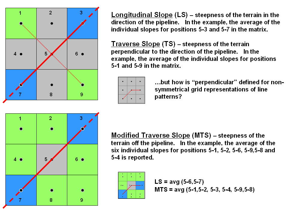
Figure 2. Modified transverse slope is calculated as
the average of off-route slopes surrounding a location.
A more radical extension considers the off-route cells in calculating Transverse Slope (TS). Traditionally, transverse slope was manually calculated by estimating the slope of a line perpendicular to the route. For example in the upper portion of figure 2, the slopes from the center cell (5) to the NE (5-3) and SW (5-7) cells identify the longitudinal slope along the route while the slopes to the NW (5-11) and SE (5-9) cells indicate the transverse slope.
The perpendicular approach works for any orthogonal and diagonal transect of the window. The elevation grid, however, can take an oblique bend involving diagonal and orthogonal directions as shown and there isn’t a true perpendicular. In this instance, GIS-derived transverse slope requires a new definition.
Modified Transverse Slope (MTS) calculates slope for the off-route cells, regardless of the linear shape. In the lower-left portion of figure 2 all of green cells (1, 2, 4, 6, 8 and 9) are considered in calculating terrain steepness surrounding the pipeline. Ideally, routes with fairly gentle modified transverse slopes are preferred as subsidence risks are lower.
These fairly innocuous extensions for calculating slope point to a bigger issue in map analysis—mainly that our grid-based analytical toolbox and GIS modeling expressions are a long way from complete. Most of the development occurred in the 1970s and 80s and coding of new capabilities in flagship systems have languished. As a result, solution providers are encoding specialized tools for their clients and running them outside the GIS or hooking them in as objects or add-ins.
What I find interesting is that this is where GIS was in the 1970s and early 80s—a collection of disparate proprietary systems. With all that you hear about data standards, open systems and GIS community access it’s peculiar that map analysis seems to be moving in the opposite direction.
Generating Mountains
and Molehills from Field Sampled Data
(GeoWorld, August 2013)
Geotechnology has revolutionized the dogma, development and
dissemination of spatial information—duh.
Today’s youth is growing up in an increasingly cyber-based society with
instantaneous connection to the world about them, and like Peter Pan they can
be whisked-away by Google Earth to distant lands in the blink of an eye.
But what if they are interested in detail beyond the maximum level of
the zoom slider bar? Or they want to
simulate localized surface flow paths, convergence and path density? Or identify subtle hummocks and
depressions? Or model subsurface
moisture regimes? Or relate any of these characteristics to the spatial
relationships with vegetative patterns?
That’s the dilemma of many aspiring scientists who want to go beyond simply visualizing a landscape to investigating system interactions that are spatially driven. But their data analysis quiver is primarily full of non-spatial analytic tools that rely on assessing and comparing the central tendencies of field collected data without consideration of the spatial distributions inherent in the data.
Two major obstacles stand in their way— appropriate spatial data and spatially aware analysis tools. Most readily downloadable data is too course for detailed scientific study, and even if it were available, most potential users are unacquainted with the quantitative analysis procedures involved.
Let’s consider the data limitation hurdle first and then see how its practical solution can spark spatial reasoning among non-GIS’ers. Suppose a budding grad student wants to develop a micro-terrain surface for a project area. Unless there is a Lidar over flight or total station survey of the area available, they will need to construct a detailed elevation surface from scratch.
First impulse is to use an inexpensive GPS unit (or Google’s GPS Surveyor app for Smartphones) to capture XYZ measurements throughout a project area. But alas, it is soon discovered that precision of the coordinates is insufficient for detailed mapping. The vertical precision in a GPS unit is characteristically less than half of that of the horizontal precision which in itself is plus or minus several meters—hardly the precision required for surface modeling.
Another possibility is to acquire sophisticated surveying equipment (transit, theodolite, laser rangefinder or GPS total station), but their costs are far too high both in terms of a tight budget and a demanding learning curve. A Dumpy level, tripod, graduated staff and a couple of meter tapes form a far more practical option (they are likely buried in an old storeroom on campus).
Dumpy levels work by precisely measuring vertical distances in a horizontal plane about a base location (figure 1). A bubble level is used to establish a horizontal plane in each quarter-circle to make sure it is level throughout the entire 360 degree swing of the instrument. An operator looks through the eyepiece of the telescope, while an assistant slowly rocks a graduated staff at a sample location and the maximum reading on the staff is recorded. Subtracting the Staff Reading from the Base Height determines the relative elevation of any measured point to a fraction of centimeter.
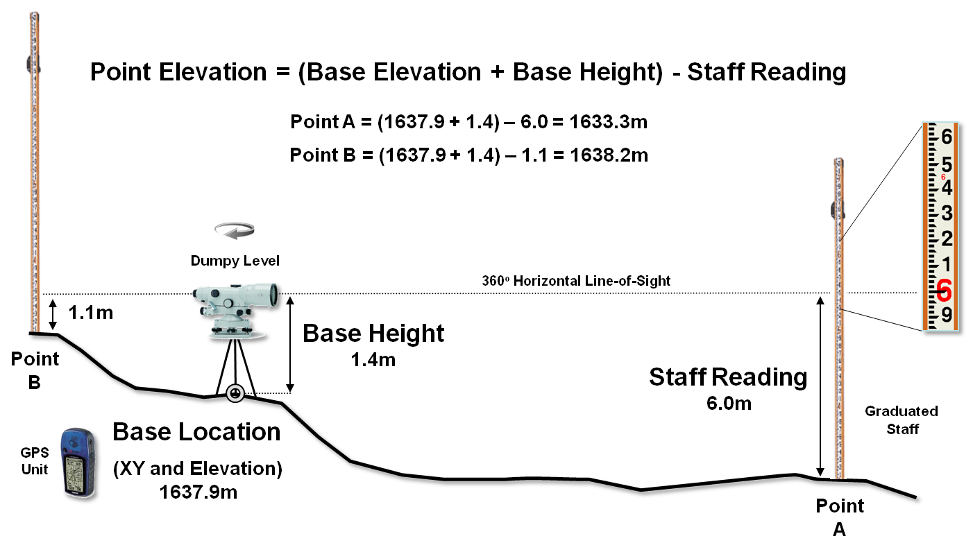
Figure 1. A Dumpy level establishes a
horizontal plane to measure the relative elevation differences throughout a
project area.
To establish real-world positioning, an inexpensive GPS unit can be used. The average of several readings taken throughout the day provides a “reasonable estimate” of the Base Location’s earth position (top-right portion of figure 2).
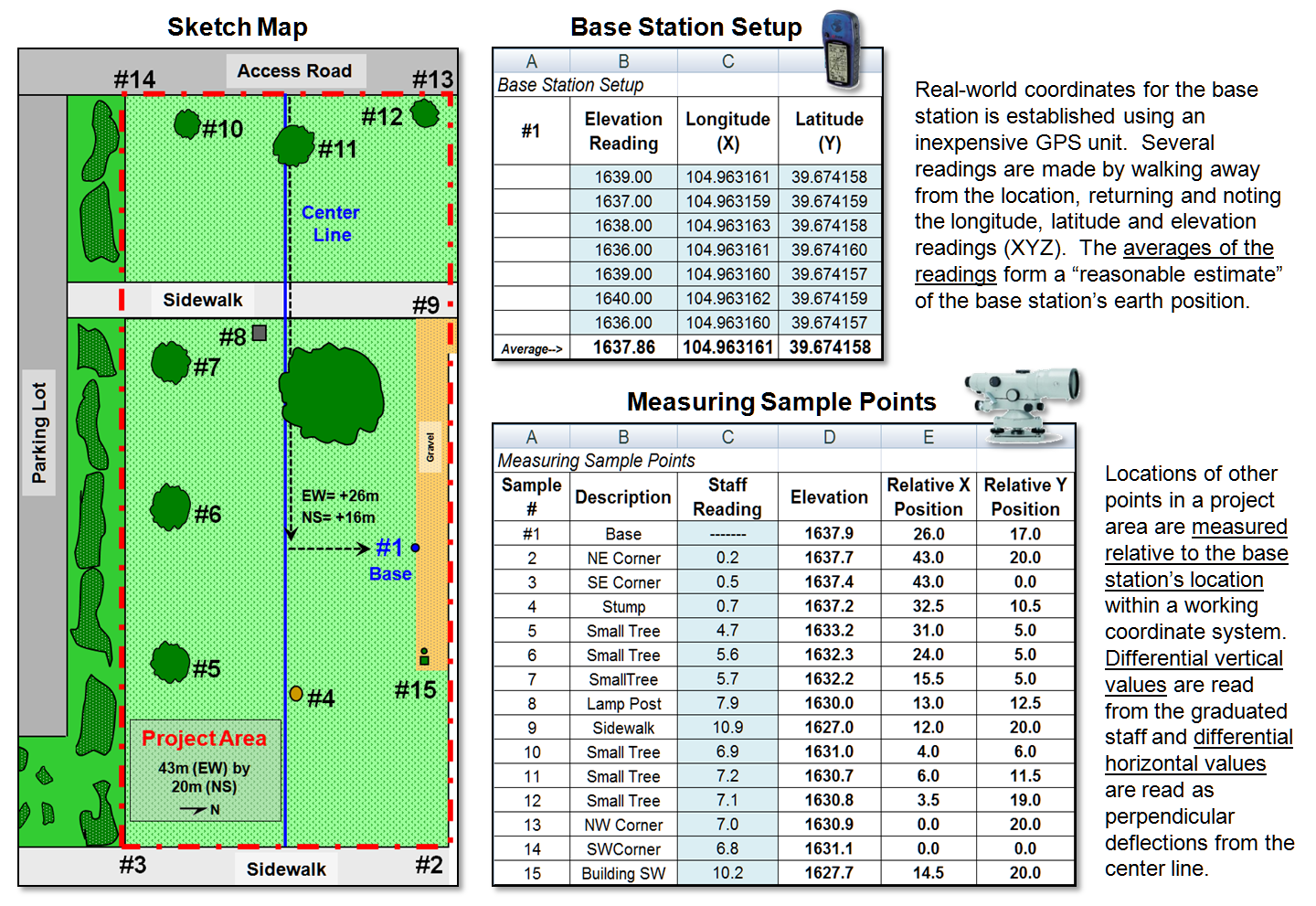
Figure 2. The XYZ coordinates of
sample points are easily derived from field data.
Before the staff is moved to another location, the distance along a center line is measured (EW as the X axis in the example) and the perpendicular deflection to the point is measured (NS as the Y axis). The result is a record of relative horizontal location and elevation difference that is easily evaluated for XYZ coordinates within a working coordinate system (bottom-right portion of figure 2) or relative to the base station’s Lat/Lon real-world coordinates.
The final step involves surface modeling software to complete the
3-dimentional surface by “spatially interpolating” the elevation values for all
of the grid cells within the project area.
Figure 3 shows the result using the powerful yet inexpensive Surfer
software package (by Golden Software).
The derived terrain surface can be exported to ArcGIS, MapCalc or other
map analysis package, as well as to Google Earth as contour lines or a
color-shaded raster image.
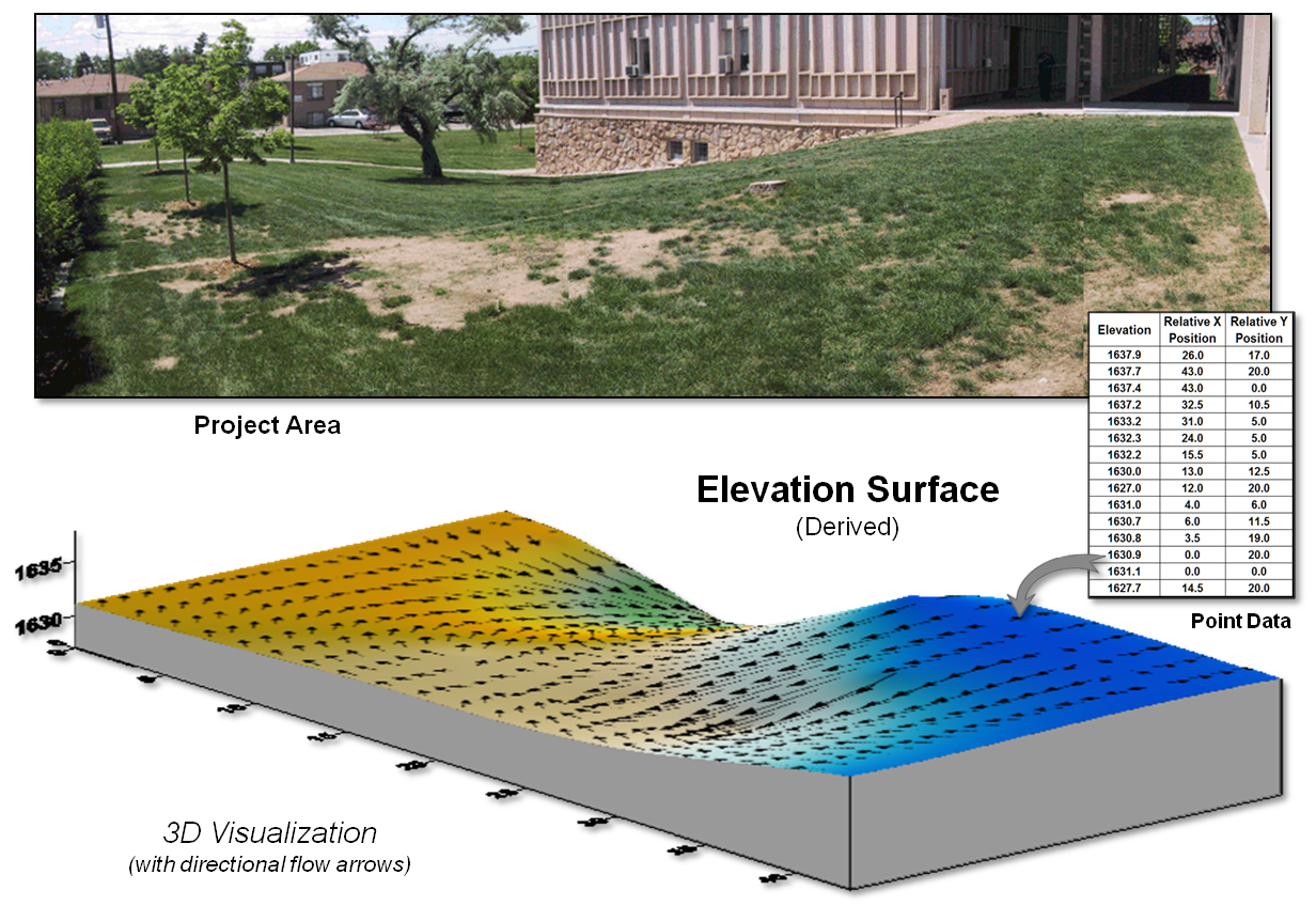
Figure 3. A detailed elevation
surface is generated using inexpensive surface modeling software.
I have presented this 3-hour workshop in various forms to numerous GIS
and non-GIS students and professionals since the 1980s. The practical fieldwork coupled with
easy-to-use software encourages dialog about the inherent spatial nature
ingrained in most field collected data.
Discussion quickly extends to data other than elevation—the “Z values”
could easily be relative concentrations of an environmental variable; or
disease occurrences in an epidemiological study; or relative biomass or stem
density measurements of a plant species; or crime incidences for mapping
pockets of crime in a city; or point of sales values for a particular product;
or questionnaire response levels in a social survey; etc.
The peaks and valleys in any map surface characterize the spatial
distribution of that mapped variable— identifying where the relative highs and
lows occur in geographic space. And
since a map surface is a spatially organized set of numbers, mathematical and
statistical analysis tools can be applied (see Author’s Note).
The bottom line is that many (most?) field-based mapped data contain
useful information about the spatial distribution/pattern inherent in the
data. While the ability to surface map
this characteristic is well-known within the GIS community, it is less familiar
and woefully underutilized in the applied sciences. A simple experience in surface mapping
terrain elevation can be useful in crossing this conceptual chasm and often
serves as a Rosetta stone in stimulating cross-discipline discussion and
recognition of “maps as data” awaiting quantitative analysis— as opposed to
traditional “graphic images” for human viewing and interpretation.
_____________________________
Author’s Note:
for more discussion on math/stat analytics for mapped data, see the online book
Beyond Mapping III, Topic 30 “A
Math/Stat Framework for Map Analysis” posted at www.innovativegis.com/basis/MapAnalysis/.
(GeoWorld, June 2007, pg. 18-19)
Dividing geographic space into meaningful groupings is the basis of all mapping. This holds for abstract maps like customer propensity clusters for purchasing a product or animal habitat suitability, as well as more traditional mapping applications such as vegetation maps, ownership parcels, highways and pipeline routes. Further divisions of the patterns in a base map often involve segmentation.
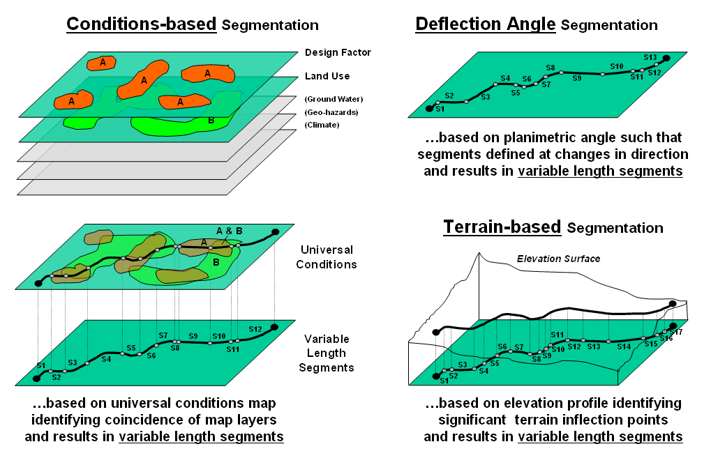
Figure 1. Basic approaches used in route segmentation.
For example, a pipeline is frequently divided into “stationing coordinates” that partitions a serpentining route into uniform linear distances along a pipeline (Uniform segmentation). Alternatively, the route can be segmented by identifying a point at each major change in direction as shown in the top right portion of figure 1. The result divides the route into a set of variable length segments responding to planimetric orientation of straight line sections (Deflection Angle segmentation).
A more complex form of segmentation is often referred to as “dynamic segmentation.” This approach uses changes in conditions on other map layers to subdivide a route. The Conditions-based segmentation procedure first derives a “universal conditions” map by overlaying a set of map layers to establish individual coincident polygons containing the same combination of conditions throughout their interiors (left side of figure 1). A route is intersected with the universal conditions map and “broken” into a series of line segments at the entry and exit of each universal condition polygon.
The result is a series of variable length line segments with uniform conditions throughout their length. The line segment set is written to a table containing x, y and z coordinates followed by fields identifying the combination of conditions along each segment. In addition, the table can report “crossing counts” that note the number of intersections of the derived line segments and other linear features, such as river and road crossings.
Another advanced form of segmentation involves breaking a route into segments considering elevation changes along a terrain surface as shown in the bottom right portion of figure 1. Terrain-based segmentation divides the route into segments representing similar terrain configuration as determined by major inflection points and slope conditions.
The first step is to establish the elevation profile of the route by “masking” the terrain surface with the route. To eliminate subtle changes, the elevation values are smoothed to characterize the overall trend of the terrain. This is done by passing a moving-average window along the elevation profile resulting in a smoothed profile.
The width of the smoothing window is critical because if it is too large the smoothing will eliminate potentially important inflection points; if it is too small there will be a multitude of insignificant segment breaks. The dilemma is similar to choosing an appropriate angular change factor in Deflection-angle segmentation and is as much art as it is science. Experience for liquid pipelines suggests an 11 to 15-cell diameter window on a 10 meter digital elevation model (DEM) works fairly well.
Figure 2. Analyzing the slope differences along a proposed route.
Figure 2 illustrates the final step in the procedure. The tool evaluates the smoothed elevation values by subtracting the current value from the previous location’s value as the solution progresses left-to-right along the smoothed profile. If the sign is the same, a continuous “running slope” is indicated. A negative difference indicates an upward incline; a negative difference indicates a downward descent; zero difference indicates no change (flat portion). A location where the sign of the difference changes (negative to positive; positive to negative) identifies an inflection point. The coordinates and elevation value for the location that changed sign is written to a Segments Table.
For example, the calculations in the upper left portion of figure 2 show a continued upward incline until the elevation point of 124 is encountered. At this location the sign of the difference changes indicating the start of a downward descent (from a negative to a positive difference).
A refinement to the approach avoids storing and processing the entire elevation profile of actual values by calculating and comparing the moving average values (smoothed elevation) on-the-fly. This approach is much more efficient and greatly improves performance. In this application a 1x15 cell window is used to smooth the actual elevation profile and store the information in a temporary table with just two records—previous and current average.
The difference is calculated and tested for a change in sign; if different, the coordinates and elevation value for the current location is written to the Segments Table. The window is advanced and the old previous average is replaced and a new smoothed value for the current location is considered. The sequence of steps of 1) replace, 2) calculate, 3) compare and 4) write if sign change is repeated until the entire profile of a route has been evaluated.
The result is a set of map segments with consistent terrain configuration. Summarizing the average slope along the segmented file provides important information for assessing the hydraulics along a pipeline and pump-station positioning and design required for anticipated product flows …a big step beyond simply mapping a pipeline route.
(GeoWorld, March 2000, pg. 23-24)
The past few columns
discussed several techniques for generating maps that identify the bumps
(convex features), the dips (concave features) and the tilt (slope) of a
terrain surface. Although the procedures
have a wealth of practical applications, the hidden agenda of the discussions
was to get you to think of geographic space in a less traditional way—as an
organized set of numbers (numerical data), instead of points, lines and areas
represented by various colors and patterns (graphic map features).
A terrain surface is organized as a rectangular "analysis grid" with
each cell containing an elevation value.
Grid-based processing involves retrieving values from one or more of
these "input data layers" and performing a mathematical or
statistical operation on the subset of data to produce a new set numbers. While computer mapping or spatial database management
often operates with the numbers defining a map, these types of processing
simply repackage the existing information.
A spatial query to "identify all the locations above 8000'
elevation in
Map analysis operations, on the other hand, create entirely new spatial
information. For example, a map of
terrain slope can be derived from an elevation surface and then used to expand
the geo-query to "identify all the locations above 8000' elevation in
Now back to business. Last month's
column described several approaches for calculating terrain slope from an
elevation surface. Each of the
approaches used a "3x3 roving window" to retrieve a subset of data,
yet applied a different analysis function (maximum, minimum, average or
"fitted" summary of the data).
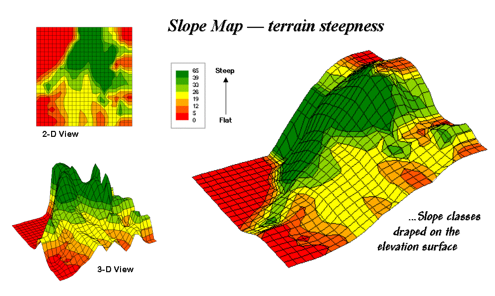
Figure 31-6. 2-D, 3-D and
draped displays of terrain slope.
Figure 31-6 shows
the slope map derived by "fitting a plane" to the nine elevation
values surrounding each map location.
The inset in the upper left corner of the figure shows a 2-D display of
the slope map. Note that steeper
locations primarily occur in the upper central portion of the area, while
gentle slopes are concentrated along the left side.
The inset on the right shows the elevation data as a wire-frame plot with the
slope map draped over the surface. Note
the alignment of the slope classes with the surface configuration—flat slopes
where it looks flat; steep slopes where it looks steep. So far, so good.
The 3-D view of slope in the lower left, however, looks a bit strange. The big bumps on this surface identify steep
areas with large slope values. The
ups-and-downs (undulations) are particularly interesting. If the area was perfectly flat, the slope
value would be zero everywhere and the 3-D view would be flat as well. But what do you think the 3-D view would look
like if the surface formed a steeply sloping plane?
Are you sure? The slope values at each
location would be the same, say 65% slope, therefore the 3-D view would be a
flat plane "floating" at a height of 65. That suggests a useful principle—as a slope
map progresses from a constant plane (single value everywhere) to more
ups-and-downs (bunches of different values), an increase in terrain roughness
is indicated.
Figure 31-7 outlines
this concept by diagramming the profiles of three different terrain
cross-sections. An elevation surface's 2nd
derivative (slope of a slope map) quantifies the amount of ups-and-downs of the
terrain. For the straight line on the
left, the "rate of change in elevation per unit distance" is constant
with the same difference in elevation everywhere along the line—slope = 65%
everywhere. The resultant slope map
would have the value 65 stored at each grid cell, therefore the "rate of
change in slope" is zero everywhere along the line (no change in
slope)—slope2 = 0% everywhere.
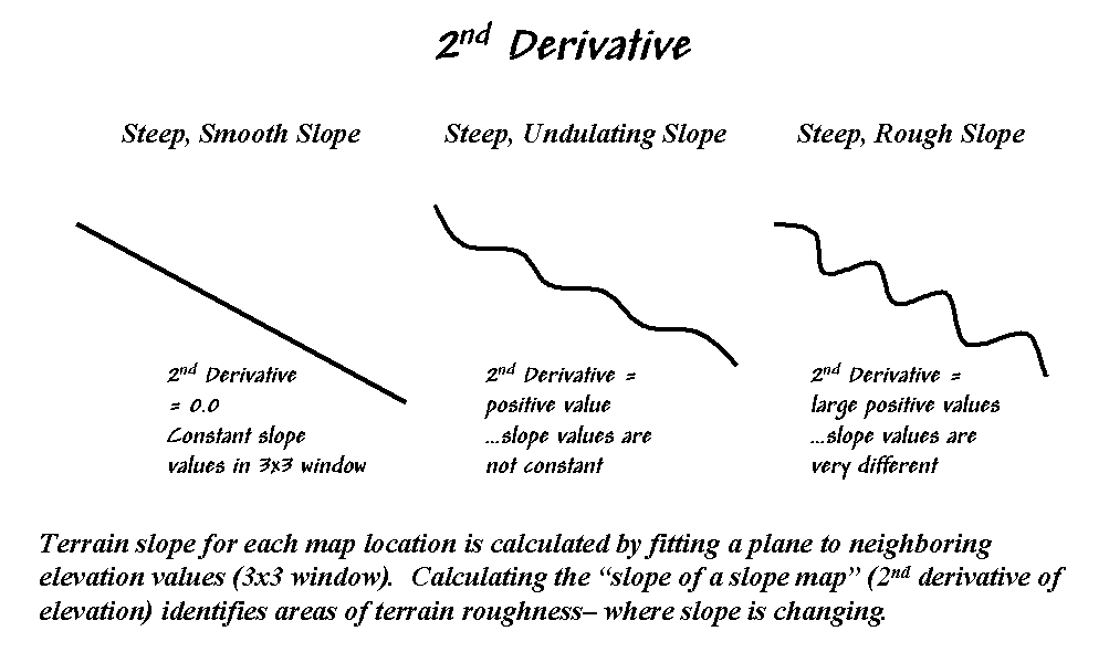
Figure 31-7. Assessing terrain roughness through the 2nd derivative
of an elevation surface.
A slope2 value of zero
is interpreted as a perfectly smooth condition, which in this case happens to
be steep. The other profiles on the
right have varying slopes along the line, therefore
the "rate of change in slope" will produce increasing larger slope2
values as the differences in slope become increasingly larger.
So who cares? Water drops for one, as
steep smooth areas are ideal for downhill racing, while "steep 'n rough
terrain" encourages more infiltration, with "gentle yet rough
terrain" the most.
Figure 31-8 shows a
roughness map based on the 2nd derivative for the same terrain as
depicted in Figure 31-6. Note the
relationships between the two figures.
The areas with the most "ups-and-downs" on the slope map in
figure 31-6 correspond to the areas of highest values on the roughness map in
figure 31-8. Now focus your attention on
the large steep area in the upper central portion of the map. Note the roughness differences for the same
area as indicated in figure 31-8—the favorite raindrop racing areas are the
smooth portions of the steep terrain.
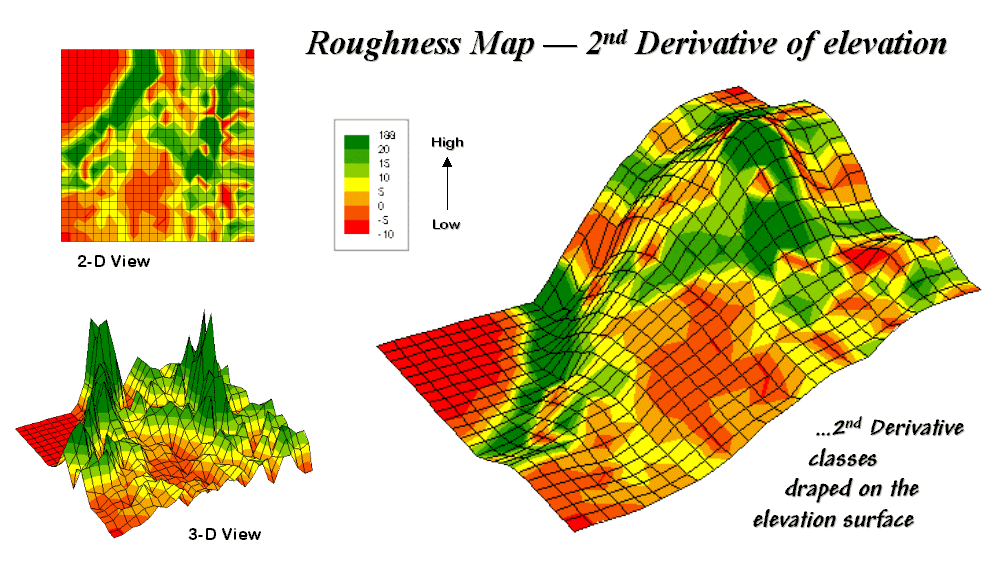
Figure 31-8. 2-D, 3-D and draped displays of terrain
roughness.
Whew! That's a lot of map-ematical
explanation for a couple of pretty simple concepts—steepness and
roughness. Next month we'll continue the
trek on steep part of the map analysis learning curve by considering
"confluence patterns" in micro terrain analysis.
Confluence Maps Further
Characterize Micro-terrain Features
(GeoWorld, April 2000, pg. 22-23)
Last section's
discussion focused on terrain steepness and roughness. While the concepts are simple and straightforward,
the mechanics of computing them are a bit more challenging. As you hike in the mountains your legs sense
the steepness and your mind is constantly assessing terrain roughness. A smooth, steeply-sloped area would have you
clinging to things, while a rough steeply-sloped area would look more like
stair steps.
Water has a similar
vantage point of the slopes it encounters, except given its head,
water will take the steepest downhill path (sort of like an out-of-control
skier). Figure 31-91 shows a 3-D grid
map of an elevation surface and the resulting flow confluence. It is based on the assumption that water will
follow a path that chooses the steepest downhill step at each point (grid cell
"step") along the terrain surface.
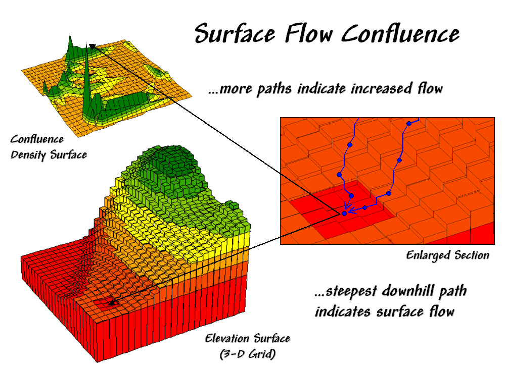
Figure 31-9. Map of surface flow confluence.
In effect, a drop of water is placed at each location and allowed to pick its
path down the terrain surface. Each grid
cell that is traversed gets the value of one added to it. As the paths from other locations are
considered the areas sharing common paths get increasing larger values (one +
one + one, etc.).
The inset on the
right shows the path taken by a couple of drops into a slight depression. The inset on the left shows the considerable
inflow for the depression as a high peak in the 3-D display. The high value indicates that a lot of uphill
locations are connected to this feature. However, note that the pathways to the
depression are concentrated along the southern edge of the area.
Now turn your attention to figure 31-10.
Ridges on the confluence density surface (lower left) identify areas of
high surface flow. Note how these areas
(darker) align with the creases in the terrain as shown on the draped elevation
surface on the right inset. The water
collection in the "saddle" between the two hills is obvious, as are
the two westerly facing confluences on the side of the hills. The 2-D map in the upper left provides a more
familiar view of where not to unroll your sleeping bag if flash floods are a
concern.
The various spatial
analysis techniques for characterizing terrain surfaces introduced in this
series provide a wealth of different perspectives on surface
configuration. Deviation from Trend,
Difference Maps and Deviation Surfaces are used to identify areas that
"bump-up" (convex) or "dip-down" (concave). A Coefficient of Variation Surface looks at
the overall disparity in elevation values occurring within a small area. A Slope Map shares a similar algorithm
(roving window) but the summary of is different and reports the
"tilt" of the surface. An
Aspect Map extends the analysis to include the direction of the tilt as well as
the magnitude. The Slope of a Slope Map
(2nd derivative) summarizes the frequency of the changes along an
incline and reports the roughness throughout an elevation surface. Finally, a Confluence Map takes an extended
view and characterizes the number of uphill locations connected to each
location.
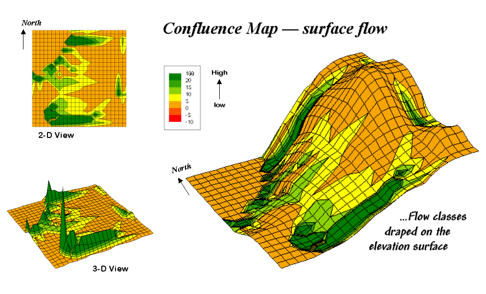
Figure 31-10. 2-D, 3-D and draped displays of surface flow
confluence.
The coincidence of
these varied perspectives can provide valuable input to decision-making. Areas that are smooth, steep and coincide
with high confluence are strong candidates for gully-washers that gouge the
landscape. On the other hand, areas that are rough, gently-sloped and with minimal confluence
are relatively stable. Concave features
in these areas tend to trap water and recharge soil moisture and the water
table. Convex features under erosive
conditions tend to become more prominent as the confluence of water flows
around it.
Similar interpretations can be made for hikers, who like raindrops react to
surface configuration in interesting ways.
While steep, smooth surfaces are avoided by all but the rock-climber,
too gentle surfaces tend too provide boring
hikes. Prominent convex features can
make interesting areas for viewing—from the top for hearty and from the bottom
for the aesthetically bent. Areas of
water confluence don't mix with hiking trail unless a considerable number of
water-bars are placed in the trail.
These "rules-of-thumb" make sense in a lot of situations,
however, there are numerous exceptions that can undercut them. Two concerns in particular are important—
conditions and resolution. First,
conditions along the surface can alter the effect of terrain
characteristics. For example, soil
properties and the vegetation at a location greatly effects surface runoff and
sediment transport. The nature of accumulated
distance along the surface is also a determinant. If the uphill slopes are long steep, the
water flow has accumulated force and considerable erosion potential. A hiker that has been hiking up a steep slope
for a long time might collapse before reaching the summit. If that steep slope is southerly oriented and
without shade trees, then exhaustion is reached even sooner.
In addition, the resolution of the elevation grid can effect
the calculations. In the case of water
drops the gridding resolution and accurate "Z" values must be high to
capture the subtle twists and bends that direct water flow. A hiker on the other hand, is less sensitive
to subtle changes in elevation. The rub
is that collection of the appropriate elevation is prohibitively expensive in
most practical applications. The result
is that existing elevation data, such as the USGS Digital Terrain Models (DTM),
are used in most cases by default. Since
the
The recognition of the importance of spatial analysis and surface modeling is
imperative, both for today and into the future.
Its effective use requires informed and wary users. However, as with all technological things,
what appears to be a data barrier today, becomes
routine in the future. For example,
The more important limitation is intellectual.
For decades, manual measurement, photo interpretation and process
modeling approaches have served as input for decision-making involving terrain
conditions. Instead of using
_______________________
Author's
Note: The figures presented in this series on
"Characterizing Micro-Terrain Features" plus several other
illustrative ones are available online as a set of annotated PowerPoint slides
at the "Column Supplements" page at http://www.innovativegis.com/basis.
(GeoWorld, May 2000, pg. 22-23)
Previous discussions
suggested that combining derived maps often is necessary for a complete
expression of an application. A simple
erosion potential model, for example, can be developed by characterizing the
coincidence of a Slope Map and a Flow Map (see the previous two columns in this
series). The flowchart in the figure
31-11 identifies the processing steps that form the model— generate slope and
flow maps, establish relative classes for both, then combine.
While a flowchart of
the processing might appear unfamiliar, the underlying assumptions are quite
straightforward. The slope map
characterizes the relative "energy" of water flow at a location and
the confluence map identifies the "volume" of flow. It's common sense that as energy and volume
increases, so does erosion potential.
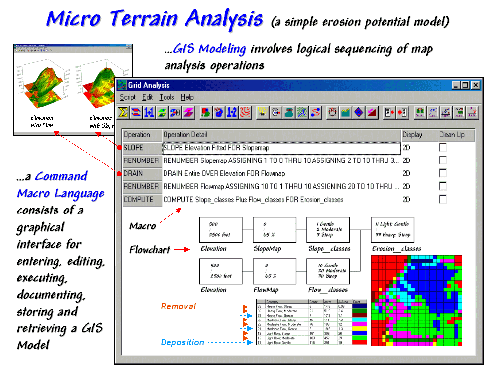
Figure 31-11. A simple erosion potential model combines information
on terrain steepness and water flow confluence.
The various
combinations of slope and flow span from high erosion potential to deposition
conditions. On the map in the lower
right, the category "33 Heavy Flow; Steep" (dark blue) identifies areas
that are steep and have a lot of uphill locations contributing water. Loosened dirtballs under these circumstances
are easily washed downhill. However,
category "12 Light Flow; Moderate" (light green) identifies locations
with minimal erosion potential. In fact,
deposition (the opposite of erosion) can occur in areas of gentle slope, such
as category "11 Light Flow; Gentle" (dark red).
Before we challenge the scientific merit of the simplified model, note the
basic elements of the
The remaining sentences in the macro and the corresponding boxes/lines in the
flowchart complete the model. The macro
enables entering, editing, executing, storing and retrieving the individual
operations that form the application.
The flowchart provides an effective means for communicating the
processing steps. Most "
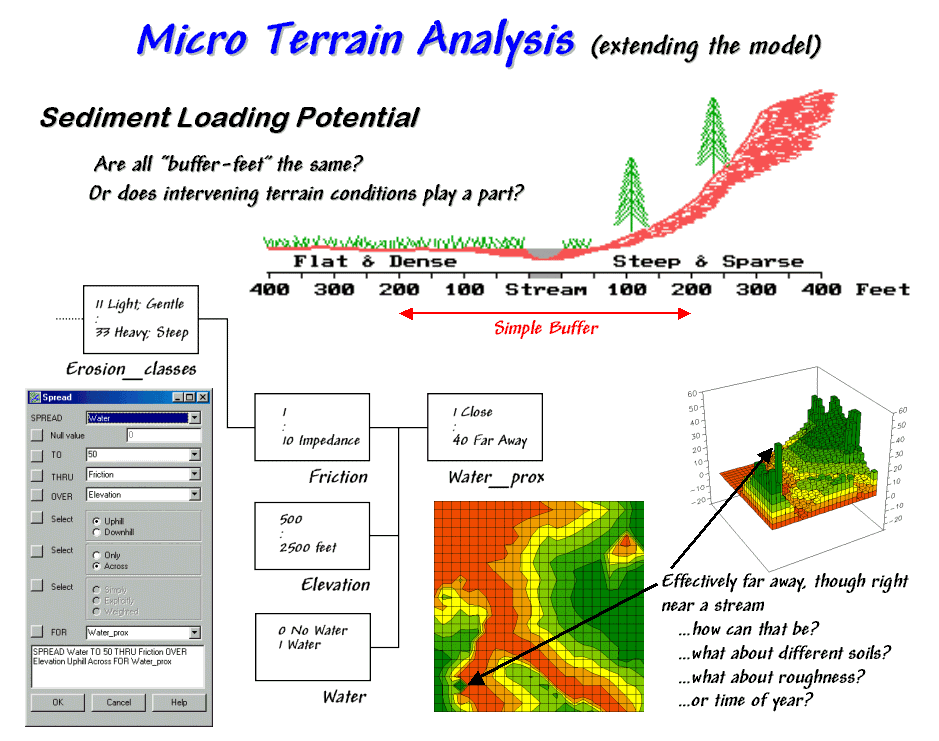
Figure 31-12. Extended erosion model
considering sediment loading potential considering intervening terrain
conditions.
It provides a
starting place for model refinement as well.
Suppose the user wants to extend the simple erosion model to address
sediment loading potential to open water.
The added logic is captured by the additional boxes/lines shown in
figure 31-12. Note that the upper left
box (Erosion_classes) picks up where the flowchart in
figure 31-11 left off.
A traditional
approach would generate a simple buffer of a couple of hundred feet around the
stream and restrict all dirt disturbing actives to outside the buffered
area. But are all buffer-feet the
same? Is a simple geographic reach on
either side sufficient to hold back sediment?
Do physical laws apply or merely civil ones that placate planners?
Common sense suggests that the intervening conditions play a role. In areas that are steep and have high water
volume, the setback ought to be a lot as erosion potential is high. Areas with minimal erosion potential require
less of a setback. In the schematic in
figure 31-12, a dirt disturbing activity on the steep hillside, though 200 feet
away, would likely rain dirtballs into the stream. A similar activity on the other side of the
stream, however, could proceed almost adjacent to the stream.
The first step in extending the erosion potential model to sediment loading
involves "calibrating" the intervening conditions for dirtball
impedance. The friction map identified
in the flowchart ranges from 1 (very low friction for the 33 Heavy Flow: Steep
condition) to 10 (very high friction for 11 Light Flow; Gentle). A loose dirtball in an area with a high
friction factor isn't going anywhere, while one in an area of very low friction
almost has legs of its own.
The second processing step calculates the effective distance from open water
based on the relative friction. The
command, "SPREAD Water TO 50 THRU Friction OVER Elevation Uphill Across For Water_Prox," is
entered simply by completing a dialog box.
The result is a variable-width buffer that reaches farther in areas of
high erosion potential and less into areas of low potential. The lighter red tones identify locations that
are effectively close to water from the perspective of a dirtball on the
move. The darker green tones indicate
areas effectively far away.
But notice the small dark green area in the lower left corner of the map of
sediment loading potential. How can it
be effectively far away though right near a stream? Actually it is a small depression that traps
dirtballs and can't contribute sediment to the stream— effectively infinitely
far away.
Several other real-world extensions are candidates to improve model. Shouldn't one consider the type of soils? The surface roughness? Or the time of year? The possibilities are numerous. In part, that's the trouble with
Identify Valley Bottoms in Mountainous Terrain
(GeoWorld, November 2002, pg. 22-23)
On occasion I am asked how I come up with ideas for the
Beyond Mapping column every month for over a dozen years. It’s easy—just hang
around bright folks with interesting questions.
It’s also the same rationale I use for keeping academic ties in
For example, last section’s discussion on “Connecting Riders with Their Stops”
is an outgrowth of a grad student’s thesis tackling an automated procedure for
routing passengers through alternative public transportation (bike, bus and
light rail). This month’s topic picks up
on another grad student’s need to identify valley
bottoms in mountainous terrain.
The upper-left inset in figure 1 identifies a portion of a
30m digital elevation model (DEM). The “floor”
of the composite plot is a 50-meter contour map of the terrain co-registered
with an exaggerated 3D lattice display of the elevation values. Note the steep gradients in the southwestern
portion of the area.
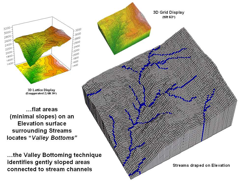
Figure 1. Gentle slopes surrounding streams are
visually apparent on a 3D plot of elevation.
The enlarged 3D grid display on the right graphically
overlays the stream channels onto the terrain surface. Note that the headwaters occur on fairly
gentle slopes then flow into the steep canyon.
While your eye can locate areas of gentle slope surrounding streams in
the plot, an automated technique is needed to delineate and characterize the
valley bottoms for millions of acres. In
addition, a precise rule set is needed to avoid inconsistencies among
subjective visual interpretations.
Like your eye, the computer needs to 1) locate areas with gentle slopes that are 2) connected to the stream channels. In evaluating the first step the computer doesn’t “see” a colorful 3D plot like you do. It “sees” relative elevation differences—rather precisely—that are stored in a matrix of elevation values. The slope algorithm retrieves the elevation value for a location and its eight surrounding values then mathematically compares the subset of values. If the nine elevation values were all the same, a slope of zero percent (flat) would be computed. As the elevation values in one portion of the 3x3 window get relatively large compared to another portion, increasing slope values are calculated. You see a steep area on the 3D plot; the computer sees a large computed slope value.
Figure 2 shows the slope calculation results for the project area. The small 3D grid plot at the top identifies terrain steepness from 0 to 105% slope. Gently sloped areas of 0-6% are shown in green tones with steeper slopes shown in red tones. The gently sloped areas are the ones of interest for deriving valley bottoms, and as your eye detected, the computer locates them primarily along the rim of the canyon. But these areas only meet half of the valley bottom definition—which of the flat areas are connected to stream channels?
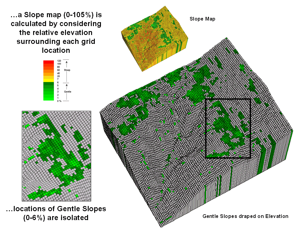
Figure 2. Slope values for the terrain surface are
calculated and gently sloped areas identified.
Figure 3 identifies the procedure for linking the two criteria. First the flat areas are isolated for a binary map of 0-6% slope=1 and greater slopes=0. Then an effective distance operation is used to measure distance away from streams considering just the areas of gentle slopes. The enlarged inset shows the result with connected valley bottom as far away as 900 meters.
While the prototype bottoming technique appears to work,
several factors need to be considered before applying it to millions of
areas. First is the question whether the
30 meter DEM data supports the slope calculations. In figure 2 the horizontal stripping in the
slope values suggests that the elevation data contains some
inconsistencies. In addition what type
of slope calculation (average, fitted, maximum, etc) ought to be used? And is the assumption of 0-6% for defining
valley bottoms valid? Should it be more
or less? Does the definition change for
different regions?
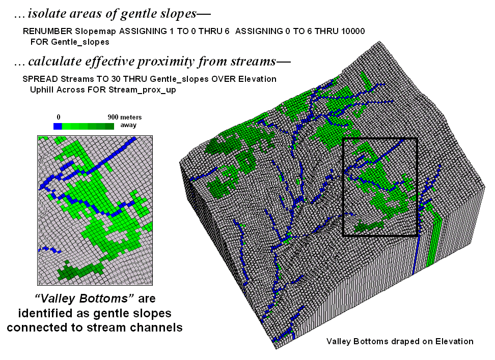
Figure 3. Valley bottoms are identified as flat areas
connected to streams.
Another concern involves the guiding surface used in
determining effective proximity—distance measurement uphill/downhill only or
across slopes? Do intervening soil and vegetation
conditions need to be considered in establishing connectivity? A final consideration is designing a field
methodology for empirically evaluating model results. Is there a strong correlation with riparian
vegetation and/or soil maps?
That’s the fun of scholarly pursuit.
Take a simple idea and grind it to dust in the research crucible—only
the best ideas and solutions survive.
But keep in mind that the major ingredient is a continuous flow of
bright and energetic minds.
_________________
Author's
Note: Sincerest
thanks to grad students Jeff Gockley and Dennis
Staley with the
Use Surface Area for Realistic Calculations
(GeoWorld, December 2002, pg. 22-23)
The earth is flat …or so most
Common sense suggests that if you walk up and down in steep terrain you will
walk a lot farther than the planimetric length of your path. While we have known this fact for thousands
of years, surface area and length calculations were practically impossible to
apply to paper maps. However, map-ematical processing in a
In a vector-based system, area calculations use plane geometry equations. In a grid-based system, planimetric area is calculated by multiplying the number of cells defining a map feature times the area of an individual cell. For example, if a forest cover type occupies 500 cells with a spatial resolution of 1 hectare each, then the total planimetric area for the cover type is 500 cells * 1ha/cell = 500ha.
However, the actual surface area of each grid cell is
dependent on its inclination (slope). Surface
area increases as a grid cell is tilted from a horizontal reference
plane (planimetric) to its three-dimensional position in a digital elevation
surface (see figure 1).
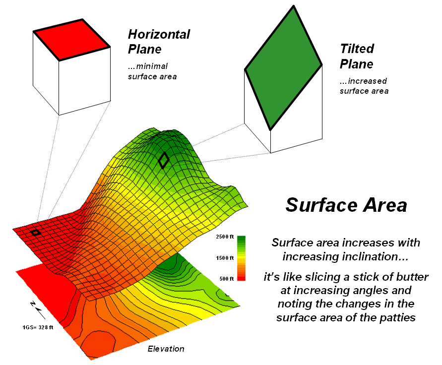
Figure 1. Surface area increases with increasing
terrain slope.
Surface area can be calculated by dividing the planimetric area by the cosine of the slope angle (see Author’s Note). For example, a grid location with a 20 percent slope has a surface area of 1.019803903 hectares based on solving the following sequence of equations:
Tan_Slope_Angle = 20 %_ slope / 100
= .20 slope_ratio
Slope_Angle = arctan (.20 slope_ratio) =
11.30993247 degrees
Surface_Area_Factor = cos (11.30993247 degrees) = .980580676
Surface_Area = 1 ha / .980580676
= 1.019803903 ha
The table in figure 2 identifies the surface area calculations for a 1-hectare gridding resolution under several terrain slope conditions. Note that the column Surface_Area_Factor is independent of the gridding resolution. Deriving the surface area for a cell on a 5-hectare resolution map, simply changes the last step in the 20% slope example (above) to 5 ha / .9806 = 5.0989 ha Surface_Area.
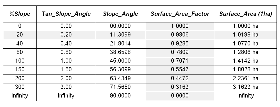
Figure 2. Surface areas for selected
terrain slopes.
For an empirical test of the surface area conversion
procedure, I have students cut a stick of butter at two angles— one at 0
degrees (perpendicular) and the other at 45 degrees. They then stamp an imprint of each patty on a
piece of graph paper and count the number of grid spaces covered by the grease
spots to determine their areas.
Comparing the results to the calculations in the table above confirms
that the 45-degree patty is about 1.414 larger.
What do you think the area difference would be for a 60-degree patty?
In a grid-based
Step 1) SLOPE
ELEVATION FOR SLOPE_
Step 2) CALCULATE ( COS
( ( ARCTAN ( SLOPE_
Step 3) CALCULATE 1.0 / SURFACE_
Step 4) COMPOSITE HABITAT_DISTRICT_
FOR HABITAT_SURFACE_
The command macro is scaled to a 1-hectare gridding resolution project area by
assigning the value 1.0 (ha) in the third step.
If a standard DEM (Digital Elevation Model with 30m resolution) surface
is used, the GRID_
A region-wide, or zonal overlay procedure (Composite), is used
to sum the surface areas for the cells defining any map feature—habitat
districts in this case. Figure 2 shows
the planimetric and surface area results for the districts considering the
terrain surface. Note that District 2
(light green) aligns with most of the steep slopes on the elevation
surface. As a result, the surface area
is considerably greater (9.62%) than its simple planimetric area.
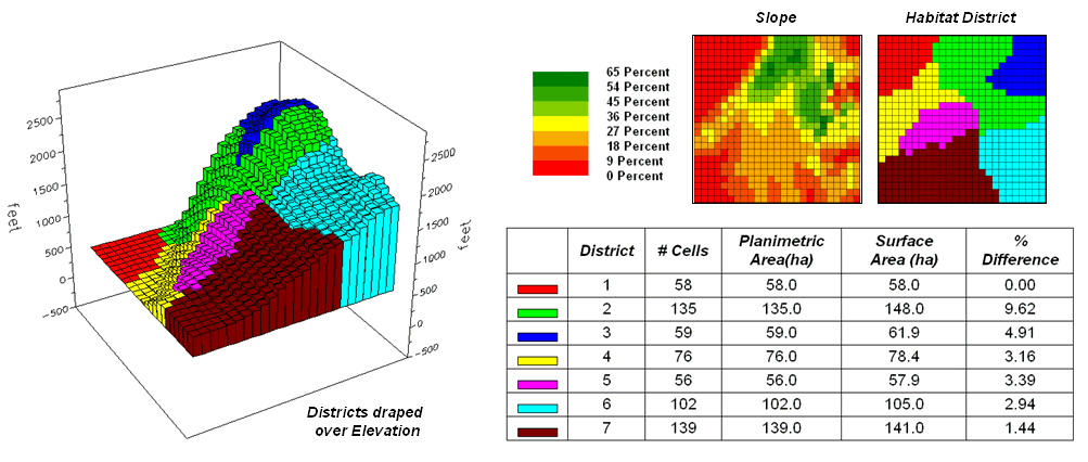
Figure 3. Planimetric vs. surface
area differences for habitat districts.
Surface length of a line also is affected by terrain. In this instance, azimuth as well as slope of
the tilted plane needs to be considered as it relates to the direction of the
line. If the grid cell is flat or the
line is perpendicular to the slope of a tilted plane, there is no correction to
the planimetric length of a line—from orthogonal (1.0 grid space to diagonal
(1.414 grid space) length. If the line
is parallel to the slope (same direction as the azimuth of the cell) the full
cosine correction to its planimetric projection takes hold. The geometric calculations are a bit more
complex and reserved for online discussion (see Author’s Note below).
So who cares about surface area and length?
Suppose you needed to determine the amount of pesticide needed for weed
spraying along an up-down power-line route or estimating the amount of seeds
for reforestation or are attempting to calculate surface infiltration in rough
terrain. Keep in mind that “simple
area/length calculations can significantly under-estimate real world
conditions.” Just ask a pooped hiker
that walked five planimetric-miles in the Colorado Rockies.
_________________
Author's
Note: For background
theory and equations for calculating surface area and length… see www.innovativegis.com/basis, select
“Column Supplements.”
Beware Slope’s Slippery Slope
(GeoWorld,
January 2003, pg. 22-23)
If you are a
skier it’s likely that you have a good feel for terrain slope. If it’s a steep double-diamond run, the timid
will zigzag across the slope while the boomers will follow the fall-line
straight down the hill.
This suggests that there are myriad slopes—uphill, across and downhill; N, E, S
and West; 0-360 azimuth—at any location.
So how can a slope map report just one slope value at each
location? Which slope is it? How is it calculated? How might it be used?
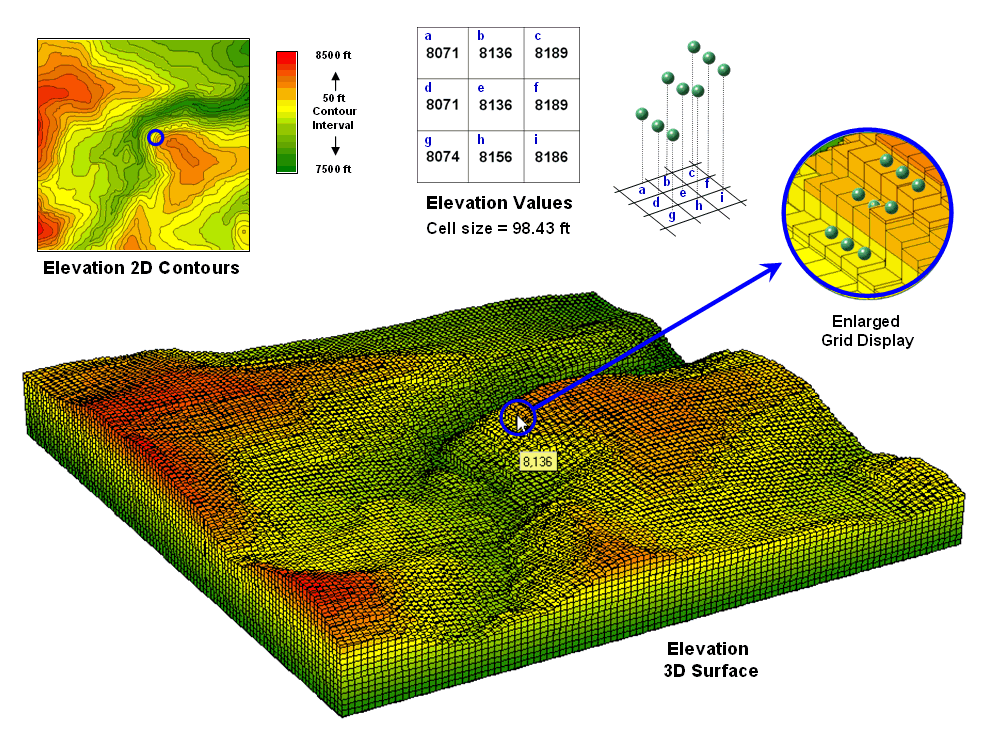
Figure 1. A terrain
surface is stored as a grid of elevation values.
Digital
Elevation Model (DEM) data is readily available at several spatial
resolutions. Figure 1 shows a portion of
a standard elevation map with a cell size of 30 meters (98.43 feet). While your eye easily detects locations of
steep and gentle slopes in the 3D display, the computer doesn‘t have the
advantage of a visual representation.
All it “sees” is an organized set of elevation values—10,000 numbers
organized as 100 columns by 100 rows in this case.
The enlarged portion of figure 1 illustrates the relative positioning of nine
elevation values and their corresponding grid storage locations. Your eye detects slope as relative vertical
alignment of the cells. However, the
computer calculates slope as the relative differences in elevation values.
The simplest approach to calculating slope focuses on the eight surrounding
elevations of the grid cell in the center of a 3-by-3 window. In the example, the individual percent slope
for d-e is change in elevation
(vertical rise) divided by change in
position (horizontal run) equals
[((8071 ft – 8136 ft) / 98.43 ft) * 100] = -66%. For diagonal positions, such as a-e, the calculation changes to [((8071
ft – 8136 ft) / 139.02 ft) * 100] = -47% using an adjusted horizontal run of SQRT(98.43**2 + 98.43**2) = 139.02 ft.
Applying the calculations to all of the neighboring slopes results in eight
individual slope values yields (clockwise from a-e) 47, 0, 38, 54, 36, 20, 45 and 66 percent slope. The minimum slope of 0% would be the
choice the timid skier while the boomer would go for the maximum slope of 66%
provided they stuck to one of the eight directions. The simplest calculation for an overall slope
is an arithmetic average slope of 38% based on the eight individual slopes.
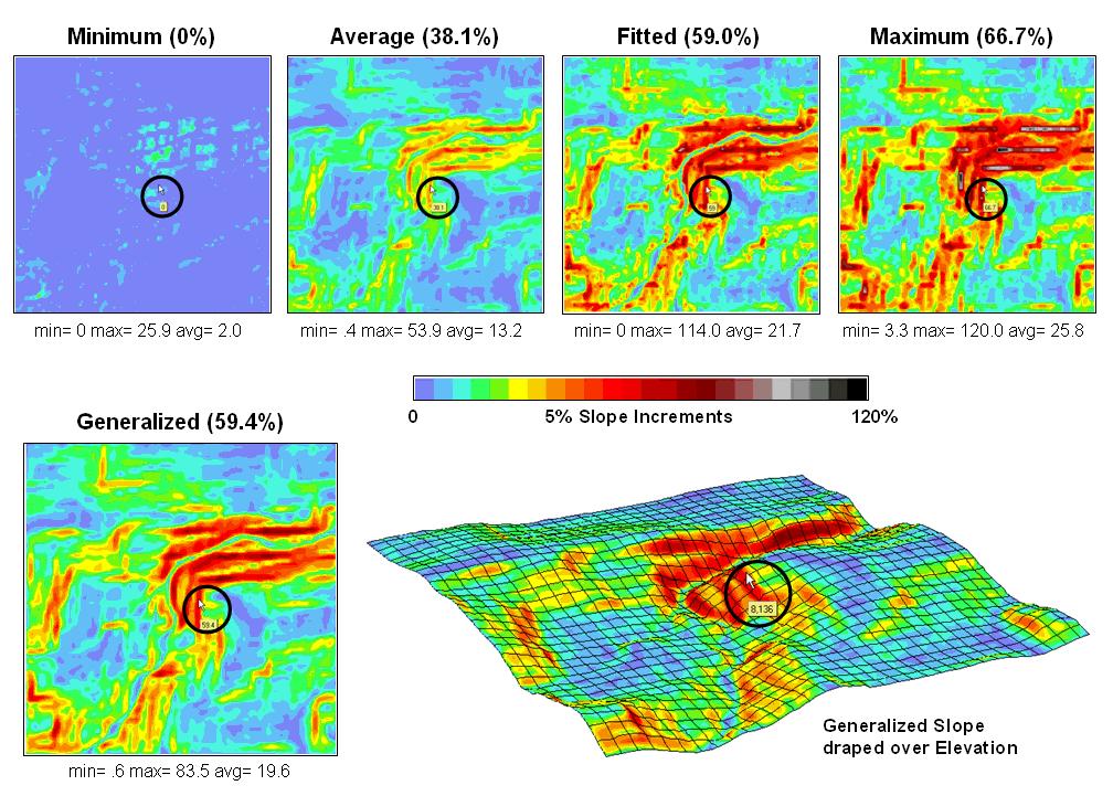
Figure 2. Visual comparison of different slope maps.
Most
The equations and example calculations for the advanced techniques are beyond
the scope of this column but are available online (see author’s note). The bottom line is that grid-based slope
calculators use a roving window to collect neighboring elevations and relate
changes in the values to their relative positions. The result is a slope value assigned to each
grid cell.
Figure 2 shows several slope maps derived from the elevation data shown in
figure 1 and organized by increasing overall slope estimates. The techniques show somewhat similar spatial
patterns with the steepest slopes in the northeast quadrant. Their derived values, however, vary
widely. For example, the average slope estimates range from .4 to
53.9% whereas the maximum slope
estimates are from 3.3 to 120%. Slope
values for a selected grid location in the central portion are identified on each
map and vary from 0 to 59.4%.
So what’s
the take-home on slope calculations?
Different algorithms produce different results and a conscientious user
should be aware of the differences. A
corollary is that you should be hesitant to download a derived map of slope
without knowing its heritage. The chance
of edge-matching slope maps from a variety of systems is unlikely. Even more insidious is the questionable
accuracy of utilizing a map-ematical equation
calibrated using one slope technique then evaluated using another.
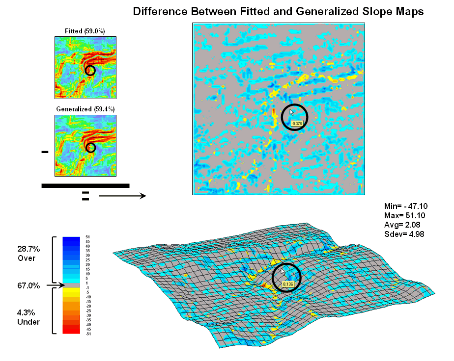
Figure 3. Comparison of Fitted versus Generalized slope maps.
The two advanced techniques result in very similar slope estimates. Figure 3 “map-ematically” compares the two maps by simply subtracting them. Note that the slope estimates for about two-thirds of the project area is within one percent agreement (grey). Disagreement between the two maps is predominantly where the fitted technique estimates a steeper slope than the generalized technique (blue-tones). The locations where generalized slopes exceed the fitted slopes (red-tones) are primarily isolated along the river valley.
Shedding Light on Terrain Analysis
(GeoWorld, April 2008,)
A lot of GIS is straightforward and mimics our boy/girl scout days wrestling with paper maps. We learned that North is at the top (at least for us in the northern latitudes) and red roads and blue streams wind their way around green globs of forested areas. However, the brown concentric rings presented a bit more of a conceptual challenge.
When the contour lines formed a fairly small circle it was likely a hilltop; or a depression, if the line sprouted whiskers. Sharp “V-shaped” contour lines pointed upstream when a blue line was present; and somewhat rounded V’s pointed downhill along a ridge. Once these and a few other subtle nuances were mastered and you survived a day or so in the woods, a merit badge and sense power over geography was attained.
Your computer is devoid of such a nostalgic experience. All it sees are organized sets of colorless numbers. In the case of vector systems, these number sets identify lines defining discrete spatial features in a manner fairly analogous to traditional mapping. On the surface, direction measurement fundamentals remain the same and your fond memory of the 0-360o markings around a compass ring holds for most GIS mapping applications.
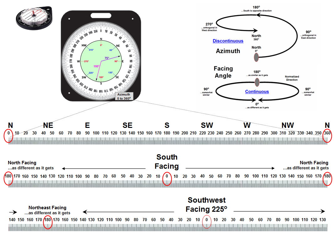
Figure 1. Azimuth is a discontinuous
numeric scale as it wraps around on itself; Facing
Angle is a continuous gradient indicating relative alignment with a specified
direction.
The upper-left portion of figure 1 unfolds the compass ring into a continuum of azimuth from 0o (north) to 360o (north). Whoa …you mean north is at both ends of the continuum? As azimuth increases, it becomes less north-like for awhile and then more north-like until 0 = 360. Now that’s enough to really mess-up a numeric bean-counter like a computer. Actually, azimuthal direction is termed a discontinuous number set as it wraps around on itself (spiral in the top-right side of figure 1).
The lower scales in figure 1 transform direction into a more stable continuous number set that indicates the relative alignment with a specified direction. A Facing Angle utilizes the concept of a back azimuth to indicate an orientation as different as it gets—180o is completely opposite; and 0o is exactly the same direction.
For a south facing location the continuum starts at 0 (South) and progresses “less south-like” in both the East and West directions until the orientation “is 180 degrees off” at due North. The importance of the consistency of this continuous scale might be lost on humans, but it means the world to a computer attempting to statistically analyze a set of directional data. The procedure normalizes terrain data for any given facing angle into a consistent scale of 0 to 180 indicating the degree of orientation similarly throughout an entire project area.
Figure 2 summarizes the geometry between Azimuth and Facing
angles. Also it introduces the concept
of a Horizontal angle that takes direction from 2D planar to 3D solid
geometry. The “Hillshade”
map of
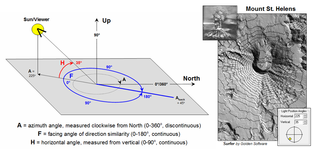
Figure 2. A Hillshade
map identifies the relative brightness at every grid location in a project
area.
Figure 3 expresses the relationship between the azimuth and horizontal angle gradients derived from aspect and slope maps. Each grid cell (30x30 meters in this example) can be thought of as a tilted plane in three-dimensional space. In the case of the brightest location, it identifies a grid cell that is perpendicular to the sun—like a contented lizard or sunbather positioned to absorb the most rays. All other possible orientations of the grid cell facets are some combination of the facing and horizontal angle gradients.
However, the “superstar map-ematicians” among us know that things are a bit more complex than an independent peek at each grid cell. A grid cell could be directly oriented toward the sun but on a small hill in the shadow of a much larger hill. To account for the surrounding terrain configuration one needs to solve the angles using solid geometry algorithms involving direction cosines to connect the grid cell to the sun and test if there is any intervening terrain blocking connection.
So what’s the take-home from all this discussion? Actually three points should stand out. First, that GIS technology encompasses our paper map thinking (e.g., discontinuous azimuthal direction), but the digital map enables us to go beyond mapping. Secondly, that a map is an organized set of numbers first, and a picture later; we must understand the nature of the data (e.g., continuous facing angle) to fully capitalize on the potential of map analysis.
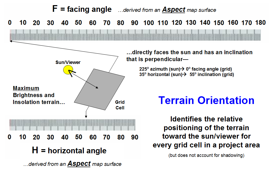
Figure 3. Terrain orientation combines azimuthal and horizontal angles for each grid cell facet.
Finally, the new map-ematical expression of maps supports radically new applications. For example, one can integrate a series of brightness maps over a day for a map of solar influx (insolation) that drives a wealth of spatial systems from wildlife habitat to global warming. In addition, these data can be statistically analyzed for insight into spatial patterns, relationships and dependencies that were beyond discovery a few years ago. In short, GIS is ushering in a new era of decision-making, not simply keeping track of where is what.
_____________________________
Author’s Note: related discussion on Terrain
Analysis is in Topic 6, Summarizing Neighbors in the book Map Analysis (
Correction:
the following letter (
Joseph—In the many years of Beyond Mapping I’ve never had a serious
disagreement. In the May column it seems as though your slant on angles is a
bit off course. I’m no map-ematician but azimuth is not discontinuous; rather it is a
cyclic attribute type that continuously wraps around (and around). If we
thought of phase angles as discontinuous we would have a hard time using sines and cosines to compute mean wind directions slope
aspects or buoy longitudes east of
Best
wishes, Peter H. Dana, Ph.D.,
Research Fellow and Lecturer, Department of Geography,
Peter—right
on …excellent points well taken. Azimuth is not “discontinuous” and your
classification of “cyclical” is a good one. The bottom line is that
azimuth isn’t your normal numerical gradient and being a bit whacko one can’t
simply utilize raw azimuth values in spatial data mining. My use of the
term “brightest areas” was misleading …I was referring to surface illumination
intensity (amount of sunlight impacting a location as contained in the facing
angle) not the relative brightness in the image which is dependent on viewer
angle as well as solar angle as compounded by the unique lay of the
terrain. Your recounting of the imaging interpretation rule also holds
true for interpreting the graphic. My point however was less on the
interpretation of the map graphic as on the ability to track solar insolation …mapped data versus visualization. The
bottom line is that I am delighted that someone out there actually reads the
column, particularly with your level of interest and expertise. The
dialog is much appreciated and I stand corrected. Thank you. Joe
Identifying Upland
Ridges
(GeoWorld, May 2009)
The good news is that there is a tsunami of mapped data out there; the bad news is that there is a tsunami of mapped data out there. Rarely is it as simple as downloading and displaying the ideal map for decision-making. More often than not the base data that is available is just that—a base for further exploration and translation into meaningful information for solutions well-beyond a basic wall decoration.
Digital Elevation Models (DEMs) are no exception. While there is an ever increasing wealth of elevation data at ever increasing detail, most applications require a translation of the ups and downs into decision contexts. For example, suppose you are interested in identifying upland ridges in mountainous terrain for wildfire considerations, wind power location or animal corridors. Downloading and displaying a set of DEMs provides a qualitative glimpse at the topography but most human interpretation becomes overwhelmed by the sheer magnitude of the possibilities and the inability to apply a consistent definition.
A topographic ridge can be defined as a long narrow upper section or raised crest of elevation formed by the juncture of two sloping planes. While the definition of a ridge is straightforward, its practical expression is a bit murkier. Figure 1 outlines a commonly used grid-based map analysis procedure for identifying ridges. The first step involves “smoothing” the surface to eliminate subtle and often artificial elevation changes. This is accomplished by moving a small “roving window” over the surface that averages the localized elevation values in the vicinity of each map location (1 Scan).
The next step simulates water falling across the entire project area and moving downhill by the steepest path (2 Drain). The computer keeps track of how many uphill locations contribute water to each grid location to generate the flow accumulation map draped over the smoothed elevation surface shown in the upper-left portion of the figure. Note that lower values (grey tones) indicate locations with minimal uphill contributors and align with the elevation crests.
The third step reclassifies the flow map to isolate the locations containing just one runoff path—candidate ridges (3 Renumber). However note the cluttered pattern of the map in the upper-right that confuses a consistent and practical definition of a ridge. The final step in the figure uses another roving window operation to assign the majority value in the vicinity of each map location thereby eliminating the “salt and pepper” pattern of the raw ridges (4 Scan). If most of the values in the window are 0 (not a potential ridge) then the location is assigned 0. However if there is a majority of potential ridges in the window then a 1 is assigned. The draped display in the lower-left confirms the alignment of the derived ridges with the terrain surface.
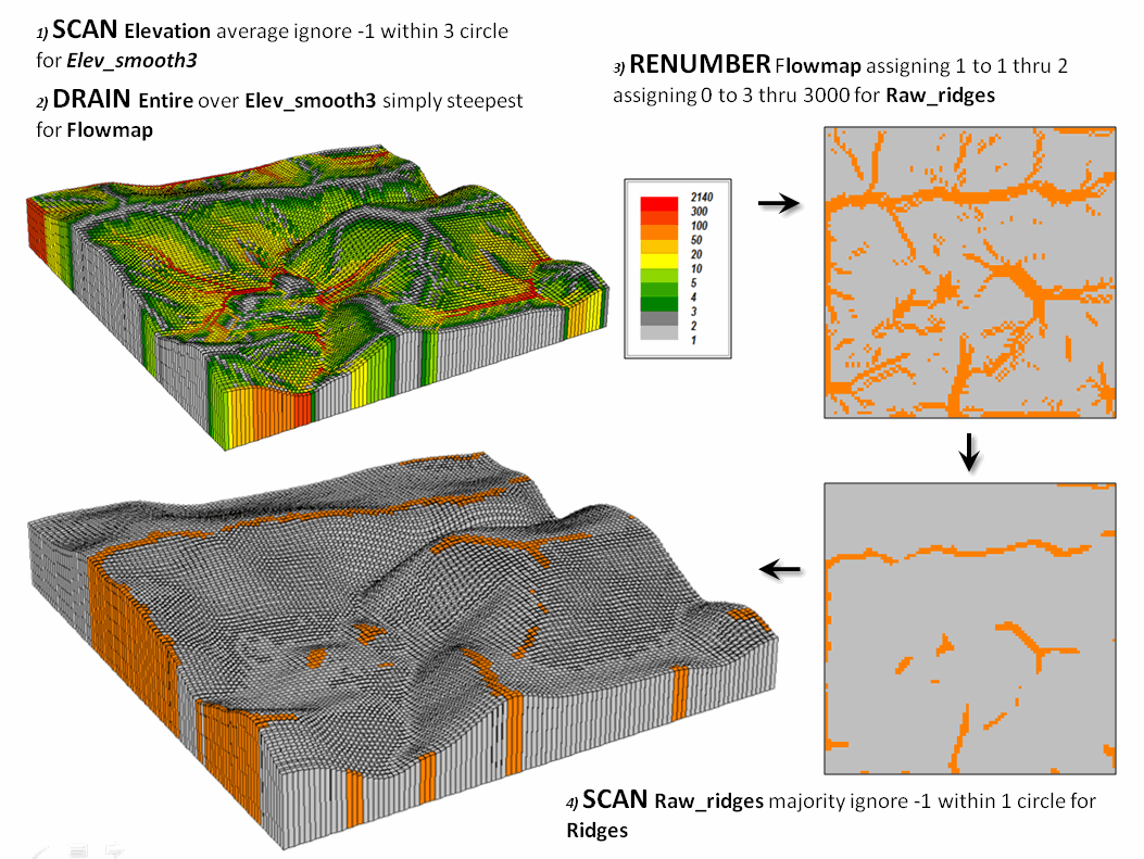
Figure 1. Accumulated surface flow is used to identify
candidate ridges.
(MapCalcTM
software commands are indicated to illustrate processing options)
Figure 2 continues the processing to identify just the upland ridges. Contiguous ridge locations are individually identified (5 Clump) and then the average elevation for each ridge grouping is determined (6 Composite). Note the low average elevation of the three small ridges in the center portion of the project area. The final step in the figure (7 Renumber) eliminates candidate ridges that are below the average elevation of the project area thereby leaving only the high ridge locations (black).
Figure 3 illustrates the processing steps for expanding the ridges as a function of terrain steepness. A slope map is generated (8 Slope) and calibrated to isolate areas of gentle slopes of 0 to 5 percent (9 Renumber). In turn, these areas are processed to eliminate the “salt and pepper” pattern (10 Scan) leaving relatively large expanses of gentle slopes.
The lower-right
map identifies the upland ridges (black) superimposed on the gently sloped
areas (red). An effective distance
operation (11 Spread) is used to
extend the ridges considering the non-gently sloped locations (grey) as
absolute barriers. The warmer tones in
the proximity map draped on the elevation surface indicate increasing distance
from a ridge into the surrounding relatively flat areas. Depending on the application the upland ridge
expansion could be reclassified from the full extent to just the immediate
surrounding areas (green).
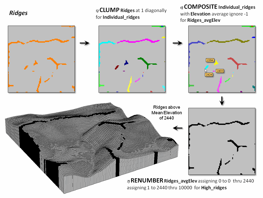
Figure 2. Low ridges are identified and eliminated.
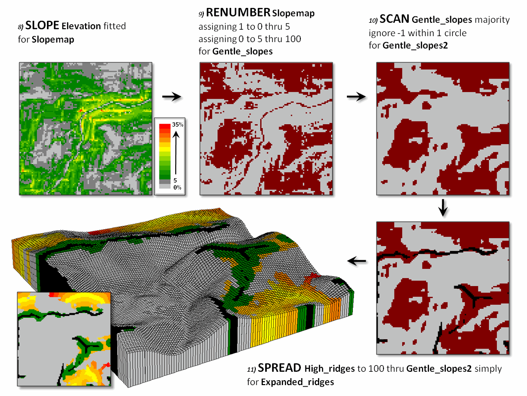
Figure 3. The ridges are extended into surrounding
gently sloped areas to identify effective upland ridges.
The simple model
may be extended to characterize conditions within the derived ridges. For example, an aspect map can be combined
with the extended ridges to indicate their overall terrain orientation or
precise azimuth each grid location defining the upland ridges to consider for
prevailing wind direction or solar exposure.
Another extension could generate an overland travel-time or a road
construction surface to consider relative access potential of the ridges.
The bottom line
is that it takes a bit of spatial reasoning to translate base maps into
decision contexts …it’s the analytic nature of GIS that moves it beyond
mapping.
_____________________________
Author’s Note: see the online book Beyond
Mapping III, Topic 11, Characterizing Micro Terrain Features at www.innovativegis.com/basis/MapAnalysis/ for additional terrain analysis techniques.
(Back to the Table of Contents)