The following is an example
graded mini-project…
Project write-up:
Landfill Suitability (use Tutor25.rgs).
The Garbage R’ Us consulting company has
approached you about sub-contracting the GIS modeling component of locating the
new land fill for
|
Criteria |
Specifications (1= worst … 9= best) |
Overall
Weighting |
|
Gently sloped |
1 = >20 percent slope 5 = 10-20 9 = <10 percent slope |
6 Times |
|
Near roads |
1 = >5 cells away 5 = 3-5 9 = <3 cells away |
2 Times |
|
Away from water |
1 = <3 cells away 5 = 3-5 9 = >5 cells away |
4 Times |
|
Not too visually
exposed to roads |
1 = >20 exposure 5 = 7-20 9 = <7 exposure |
1 Times |
|
Not in areas of
high housing density (total; within 3) |
1 = >12 houses 3 = 6-12 7 = 3-6 9 = <3houses |
2 Times |
|
On appropriate
soils |
0 = 0 open water 1 = 4 upland 3 = 1 floodplain 7 = 3 terrace 9 = 2 lowland |
8 Times |
|
|
|
|
|
Steepness
constraint |
1 = <50 percent slope
(OK) 0 = >50 percent slope
(Illegal) |
Legal Imperative |
|
Proximity to
water constraint |
1 = >1 cells away (OK) 0 = <1cells away
(Illegal) |
Legal Imperative |
Your charge is to
prepare a prospectus for deriving the Landfill Suitability map that clearly
explains how each of criteria are evaluated and then combined into an overall
suitability map that respects the legal constraints and reflects the county
commissioners’ criteria weightings.
In addition,
calculate the average landfill suitability rating for each district (Districts map). Finally, generate a map that identifies the
average rating within 300 meters (3-cell reach) for each of the housing
locations (Housing map).
_________________________________________________
Student Report:
Slippery
Mountain County
Landfill
Suitability Study
…nice graphic
A
spatial analysis
using
grid-based
to locate suitable sites for a new landfill,
A Report By: Anonymous
135.0/150 A- …very good job. Good organization and generally well-presented
…professional. The flowchart in the text
is more appropriate for the appendix …too detailed to be an overview of the
solution. Need to include some of the
important graphics (maps) in the text discussion. Additional Considerations section is
weak. Also, the Conclusion shouldn’t
introduce new material (graphics), but summarize and conclude the information
in the body of the prospectus. Very well
organized Appendix.
February 23, 2004
GEOG 3110 –
Professor: Dr. Joseph
Berry
TABLE OF CONTENTS
![]()
Introduction Page
1
Approach Page
1
Data Requirements Page
3
Prototype Model Page
3
Flowchart of Suitability
Study Page
4
Additional Considerations Page
7
Conclusions Page
8
Appendix
A Page
11
Detailed
Landfill Suitability Flowchart Page
12
Sections
on Detailed Map Analysis and Processing Functions
Section
1 – Slope Analysis Page
13
Section
2 – Road Proximity Analysis Page
14
Section
3 – Water Proximity Analysis Page
16
Section
4 – Road Visibility Analysis Page
18
Section
5 – Housing Density Analysis Page
19
Section
6 – Soils Analysis Page
21
Section
7 – Steepness Constraint Page
22
Section
8 – Water Constraint Page
22
Section
9 – Total Suitability Maps Page
23
Section
10 – Final Suitable Landfill Locations Page
24
Section
11 – Average Suitability Rating for Districts Page
27
Section
12 – Housing Rating Within 300 meters Page
28
…the page numbers in the T of C work for hardcopy printout,
but not for an electronic report (particularly after I have messed with it)
…would be more 21st century to hyperlink using
bookmarks. I made the Appendix item in
the T of C hyperlinked to a book mark by highlighting the Title “Appendix” then selecting Insertà Bookmarkà and naming it “Appendix”; then highlighted the item “Appendix” in the T of C and pressing
the Hyperlink buttonà pressing the Bookmark
buttonà selecting the item “Appendix”
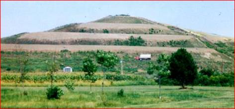
INTRODUCTION
The population of
With the substantial increase in population and new
businesses over the past 5 years, this has put a tremendous strain on the
counties current landfill space. The
county currently has only 1 landfill for all of its residents, and the current
landfill is expected to reach capacity within the next 3 to 5 years.
Garbage R’ Us consulting company, one of the nations
leading companies for developing and locating potential new landfill sites, has
recently approached our company, LGIS (Landfill
…might be useful to mention the drawbacks of current manual
map analysis procedures that they are using
APPROACH
Garbage
R’ Us , LGIS, and the county commissioners had a “kickoff meeting” to discuss
what factors they thought were most important in finding a suitable location
for a new landfill prior to getting started with the study. The county commissioners over the past
several months have received numerous letters from concerned citizens and many
citizens have voiced concerns at county commissioner meetings over the new landfill. There were many different factors discussed
and it was difficult for the group to come to a consensus on what factors were
the most important ones.
The
factors that the group agreed were the most important ones are listed in Figure
1 below. These factors do not represent
all of the possible factors that could be considered, but are considered the
most critical factors and the factors on which information is most readily
available from the counties current
![]()
Slippery Mountain County
Landfill Suitability Study
Page 1 …20th century page Print
orientation; soon will go the way of the punch card, but still useful if a
printed report is the objective
The
6 criteria used in our analysis are listed in Figure 1 below and 2 constraint
criteria (steepness and proximity to water) are also listed in Figure 1.
|
Criteria |
Specifications ( 1
= worst, …….9 = best) |
Overall Criteria Weighting |
|
Gently
Sloped Area |
1
= > 20% Slope 5
= 10-20 % Slope 9
= < 10 % Slope |
6
Times |
|
Near
Roads |
1
= > 5 cells away 5
= 3-5 cells away 9
= < 3 cells away |
2
Times |
|
Away
From Water |
1
= 0-3 cells away 5
= 3-5 cells away 9
= 5 cells away |
4
Times |
|
Not Too Visually
Exposed to Roads |
1
= > 20 cell exposure 5
= 7-20 cell exposure 9
= < 7 cell exposure |
1
Times |
|
Not in Areas of High
Housing Density (total; within 3) |
1
= > 12 houses 3
= 6-12 houses 7
= 3-6 houses 9
= < 3 houses |
2
Times |
|
On
Appropriate Soils |
0
= 0 open water 1
= 4 upland 3
= 1 floodplain 7
= 3 terrace 9
= 2 lowland |
8
Times |
|
|
|
|
|
Steepness
Constraint |
1
= < 50% slope (OK) 0
= > 50% slope (illegal) |
Legal
Imperative |
|
Proximity
to Water Constraint |
1
= > 1 cells away (OK) 0
= < 1 cells away (illegal) |
Legal
Imperative |
Figure 1 – Landfill Suitability Criteria and
Overall Weighting for Criteria
The LGIS solution
uses… present tense is a bit more optimistic LGIS will use the
The
criteria represented in Figure 1 are
the criteria that the county commissioners and the consultants (LGIS and
Garbage R’ Us) agreed upon and these criteria have data readily available for
them. The specifications section of the
table assigns a rating for each of the 8 criteria. A rating of 1 for the gently sloped areas for
instance indicates that a slope greater than 20% is the worst while a 9 value
indicates that a slope value of less than 10% is the best. Then each criteria is multiplied by a
weighting factor since some criteria are deemed as more important that
others. Gently sloped areas have a
weighting factor of 6, while the near roads criteria criterion has a weighting
factor of 2. When the
![]()
Slippery Mountain
The criteria listed in Figure 1
represent the base data files that we will use for conducting our suitability
analysis for the new landfill. These
criteria were considered the most important criteria and are the criteria for
which
The study area for our demonstration analysis is a 25 cell by 25 cell (2,500 meter
by 2,500 meter) area in the southwest corner of
PROTOTYPE
MODEL
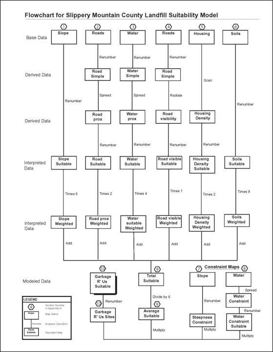
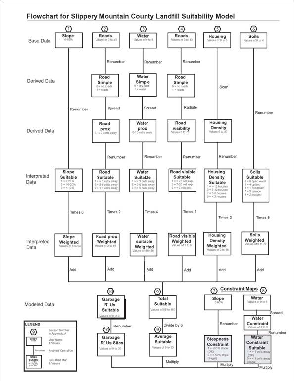
The flowchart in Figure 2 shows the
process that LGIS went through to find a suitable location for a new
landfill. Our discussion will be more
general in nature and will focus more on the process and general discussion of
the model that we used. Specific details
on processing operations and commands used to implement the model can be found
in Appendix A of this report. A more
detailed flowchart can also be found in Appendix A on page 12.
1.
Base Data Maps
For our suitability analysis, we used 6 different
criteria as shown in Figure 1. These 6
criteria represent base data that we obtained from
2. Derived Data Maps
Since the base data in and by itself is not of much use
to us in determining a suitable location to build a new landfill, we will need
to manipulate and analyze the data to produce the desired outcomes. The derived data maps as shown in the
flowchart in Figure 2 are maps that are generated from the base data maps. We do this to simplify the data on the base
maps (such as to aggregate values) and to find areas of interest in our study
area (such as locations within 1,000 meters of a road). Note that we are not changing any of the
original data on the base maps, we are simply changing the display
characteristics of the data.
![]()
Slippery Mountain
 …too detailed for
the general approach section---more in tune with the Appendix
…too detailed for
the general approach section---more in tune with the Appendix
Figure 2 – Flowchart for the Slippery
![]()
Slippery Mountain
Described
below are some of the specific details of the derived data maps used in our
suitability study and the information that they provide us with.
- Roads Simple Map – A zero value
means no roads are present, a 1 value means that a road is present
- Water Simple Map – A zero value
indicates dry land, a 1 value indicates a water feature
- Road Prox Map – Shows all
locations with 10 cells (1,000 meters) of a road
- Water Prox Map – Shows all
locations within 10 cells (1,000 meters) of a water feature
- Road Visibility Map – Identifies
how many times a location is seen from each location (cell) on each of the
roads for all of the roads in the study area
- Housing Density Map – Identifies
how many houses there are for a particular location (grid cell) on the map
Although
the derived data maps described above provide us with more useful information
than the base data maps, this information still is of little use to us since we
really have not defined if a particular location or area is more important than
another. We may for instance really want
to put a landfill within 3 cells of a road and a distance of 10 cells away from
a road would be too far away to put a new landfill.
3. Suitability Maps
In order to remedy our problem described in the previous
paragraph, we used a rating suitability model to determine the most suitable
area(s) for a new landfill. In this
particular type of model, we assign a “goodness scale” to the criteria we
specified in Figure 1. The goodness
scale in our model has values ranging from 0 to 9. A zero value in this scale represents a
constraint, meaning that it is either physically impossible to build a landfill
at that location or that the laws of
The 1 thru 9 values on the goodness scale represent how
suitable a location is based on our specified criteria. For this model, we use the following numbers
and “ratings” in Figure 2 to determine locations suitability for a new
landfill.
|
Value |
Rating |
|
1 |
Poor |
|
3 |
Fair |
|
5 |
Good |
|
7 |
Very
Good |
|
9 |
Excellent |
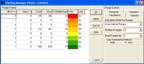
Figure 3 – The Goodness Scale for
Suitability …not sure this warrants a table
![]()
Slippery Mountain
The
specific suitability values as described in Figure 1 for each of the 6 criteria
are listed and described in more detail below.
Note that 1 cell is equal to a distance of 100 meters and that the terms
“cells” and “locations” are used interchangeably.
- Suitable Slopes Map – 1 for slopes
over 20%, 5 for slopes 10-20%, and
9 for slopes under 10%
- Suitable Roads Map – 1 for
locations 5 cells or more away from roads, 5 for locations 3 to 5 cells
away, and 9 for locations within 3 cells of a road
- Suitable Water Map – 1 for
locations within 3 cells of a water feature, 5 for locations within 3 to 5
cells of a water feature, and 9 for locations 5 or more cells away from a
water feature
- Suitable Housing Density Map – 1 for
locations with a density of 12 or more houses, 3 for locations with 6 to
12 houses, 7 for locations with 3 to 6 houses, and 9 for locations with a
housing density of less than 3 houses
- Suitable Soils Map - 0 for locations with open water (lakes,
etc.), 1 for upland type soils, 3 for floodplain type soils, 7 for terrace
type soils, and 9 for lowland type soils
All
of the maps listed above will display data in a range of values from 0 to
9. A zero value represents a constraint
while a 9 value represents the highest suitability (an excellent area).
Keep
in mind that these numbers and the ratings assigned to them were chosen by LGIS
to conduct the analysis. Limiting the
number of values we use for the analysis will make the model easier to run and
will make the results more understandable for the county commissioners and the
general public. One problem with this
approach is that a location may not exactly fall into one of the given values
in the chart in Figure 3. A location or
locations for instance may have a value of 6, which would fall between the good
and very good ratings shown in Figure 3.
In this situation, LGIS will need to make a judgment call as to whether
the area would receive a “good” or a “very good” rating. This “goodness scale” will then be applied
with the weighting criteria factor discussed in the next paragraph of this
report to generate a final suitability map.
<blank line>
4. Weighted Suitability Maps
The saying “all things
are not created equal” certainly applies to building a
By assigning a weight to each of the 6 criteria in our
model (see Figure 1), we put more or less emphasis on a particular criteria in
the model. The “soils” criteria for
instance are assigned a weight of 8, meaning that it will have the highest
level of importance in our final suitability map. Road visibility for instance will be assigned
a weight value of 1, meaning that it will have the lowest level of importance
in our final map. The higher the weight
value for a particular criteria criterion in our model, the more a particular
criteria will influence the final suitability map in our model. The suitability maps described above are
multiplied by the weight factor to determine the weighted value for each
map. Provided below is a more detailed
description of the weighted maps we generated and the values for each map.
![]()
Slippery Mountain
·
Slope Weighted Map – Multiply the Suitable Slopes Map by 6. Values on this map range from 6 to 54
·
Road prox Weighted
Map –
Multiply the Suitable Road Prox Map by 2.
Values on this map range from 2 to 18
·
Water Suitable
Weighted
Map– Multiply the Water Suitable Map
by 4. Values on this map range from 4 to
36
·
Road Visible Weighted
Map –
Multiply the Suitable Road Visibility Map by 1.
Values on this map range from 1 to 9
·
Housing Density
Weighted Map –
Multiply the Suitable Housing Density Map by 2.
Values on this map range from 2 to 18.
·
Soils Weighted Map - Multiply the Suitable Soils Map by 8. Values on this map range from 0 to 72
On
the weighted maps, a higher number indicates a higher suitability. The values on the weighted maps range from a
zero (constraint area) to a 72 (very high suitability).
…composite graphics might be useful to “show” the groups of
maps
<blank line>
5. Add the Weighted Suitability Maps Together
and Find the Average Suitability
The 6 weighted suitability maps listed in the previous
section are added together to produce a total suitable map. The total suitable map we generated has a
range of values from 55 to 183. The
possible range of values on this map could be from 15 (the sum of all the
lowest values on each of the 6 weighted maps) to 197 (the sum of all of the
highest values on each of the 6 weighted maps).
This means that there are no areas that are totally poor or unbuildable
( areas with a value of zero or 15) or areas that are totally excellent (with a
value of 197) for locating a landfill.
However we need to find the average suitability for each
location and to do this we needed to divide the total suitable map by 6 since
the total suitable map is the sum of the 6 weighted suitability maps to derive
the average suitable map. The average
suitable map has values ranging from 9 to 33, with a 9 value representing the
poorest suitability and a 33 value representing the highest suitability.
…would be useful to show some of the more/most important
solution map (figure 5?)—or hyperlink to the displays in the Appendix
5.
Constraint Maps
No matter what type
of study or analysis you are doing, there are always those factors that make
what you are trying to do impossible or not feasible. In our landfill study model, we determined
that very steep slopes and areas that have water features and are in very close
proximity to water areas would make it impossible to build there. This is due to either legal constraints (the
county won’t allow it) or it’s physically impossible to do so (like putting a
landfill in the middle of a lake or on a very steep slope where all of the
trash could slide off). The constraint
maps will allow us to mask out those areas where it is impossible or illegal
for us to locate a new landfill. The
constraint maps in our model are as follows:
·
Steepness Constraint
Map –
A zero value represents those areas where the slope is greater than 50%.
·
Water Proximity
Constraint Map –
A zero value represents an area that is less than 1 cell away from a water
feature and includes areas that have a water feature, such as a lake. This is a legal requirement of
·
???
![]()
Slippery Mountain
6.
Garbage
R’ Us Suitable Sites
The
final step in our analysis is to take the average suitable map and to multiply
this map with the steepness and water proximity constraint maps. Since the non-buildable or illegal areas on
the constraint maps have a value of 0, when we multiply the constraint maps
with the average suitable map, we will end up with a value of 0 on the Garbage
R’ Us Suitable Sites Map (since 0 times any value = 0) for all those areas
where it is impossible or illegal to build a new landfill. The 1 values on the constraint maps will have
no effect on the average suitable map values since any value on that map
multiplied by 1 will result in the same value on the Garbage R’ Us Suitable
Sites Map.
The
Garbage R’ Us Suitable Sites Map shows us values ranging from 0 (non-buildable
areas) to a 30 (highly suitable). We
renumbered these range of values to work with our suitability rating system (1
= poor…..9 = excellent) using the following breakdown of values.
…need a graphic (map) of the result
|
Value |
Rating |
|
|
0 |
Non-Buildable
/ Illegal |
0 |
|
1 |
Poor |
1
to 9 |
|
3 |
Fair |
9
to 15 |
|
5 |
Good |
15
to 21 |
|
7 |
Very
Good |
21
to 27 |
|
9 |
Excellent |
27
to 30 |
Figure 4 –
Suitability Rating System for the Garbage R’ Us Suitable Sites Map
ADDITIONAL
CONSIDERATIONS
The criteria we used
to run our suitability model for a new landfill do not represent the only
criteria that we could have used for our study.
We for instance did not look at potential rare or endangered plant or animal species
that may be present in the study area.
Rare and endangered plant and animal species could potentially kill any
potential project depending on how limited of a habitat these species may
have. Our model also does not look at
potential noise impacts
from the increased amount of trucks and heavy machinery that would be using the
landfill on a daily basis. Perhaps more
importantly than anything else is that the suitability model that we run should
be field verified. The
A model is a work in progress and undergoes several changes and
levels of refinement before the model is finalized. In fact the model may never be truly
finalized since additional information, citizen input, and changing needs or
requirements over time may effect how the model is run and would change the
desired outcomes. …true but might
scare the client The model also needs to be flexible and
adaptable to changes as they arise over time.
…other extensions might be to incorporate visual exposure to
houses; simple proximity (or downwind proximity) to houses (roads); section
should
![]()
Slippery Mountain
CONCLUSIONS
Through our analysis and running of our
model, we found a total of 8 sites that would receive an excellent rating in
our model (a suitability rating of 27 or higher) as shown in Figure 5a
below. 5 of these locations were single
cell (100 m x 100 m) locations where it would not be practical to build a new
landfill. The largest continuous location
is at the bottom left corner of the map in Figure 5a colored in red had an area of 49.4 acres. The tan colored areas directly above this
area with a “very good” rating makes up another 46.9 acres. The grey colored areas on the map in Figure
5a represent those areas where there were constraints (steepness and proximity
to water) and the red colored areas represent those areas that are
excellent. The tan colored areas on the
map are areas with a “very good” rating, and many of these areas are directly
adjacent to the areas colored in red with an excellent rating. Note that on the final map there are no
“poor” areas since the Garbage R’ Us suitability map had no values in the range
of 1 to 9.
The
map in Figure 5b shows us the suitability when we clump areas together with
similar values. We use the criteria
specified in Figure 4 to renumber the map to 0 thru 9 values. The black areas on this map represent
constraint areas and areas with a suitability rating of less than 7. The large red area on this map for instance
has an area of 227 acres. More detail on
how the map in Figure 5b is derived is provided in Section 10 of Appendix A on
page 24. The important thing to note is
how you display the data and group the values together can have a substantial
effect on what areas are analyzed as being suitable.
We also discovered that the district with the highest
suitability rating was district 6, with an average rating of 4.78 (using the 0
to 9 suitability scale) while district 1 had the lowest rating with a value of
zero (not buildable since this district is a lake). See Section 11 in Appendix A on page 27 for
the data maps used and the processing operations used. For the average suitability rating within 300
meters (3 cells) of the housing locations, we found that all of the houses
happened to lie in fairly suitable areas with the range of values being from
5.08 to 5.81 on the suitability scale from 0 to 9 with 9 being excellent and 0
being non-buildable. See Section 12 in Appendix A on page 28 for more
information on the analysis and processing operations used.
The results of our analysis show that our study area has
several “very good” to “excellent” areas for locating a new landfill. This map represents a good staring point and
it helps us to narrow down our list of potential sites for a new landfill. Through citizen input, field visits, and
additional studies,
![]()
Slippery Mountain
A. Garbage_R_Us_Sites Map B.
Garbage_R_Us_Siteareas Map
…better presented in a 2x2 table; use of cryptic map names
isn’t appropriate for the overview
…useful to have some annotations that “pull” the reader into the points you
want to make with these fifures
Figure 5 –
Garbage R Us Sites Map and Garbage R Us Site-areas Maps (with clumped areas)
Showing the Most Suitable Locations for a New Landfill …these need
to be in the body
![]()
Slippery Mountain
Figure
6 - Detailed Flowchart for the Slippery
![]()
Page 12
Provided in the following 12
sections of this appendix are detailed descriptions of the map analysis
operations used and graphical displays of the intermediary maps and command
dialog boxes used to complete the analysis.
Note: All specific commands used are in capital
letters and boldface type.
1. Slope Analysis
…Step ??? in the flowchart— could relate to
flowchart
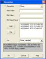
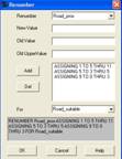
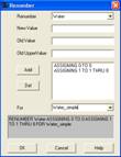
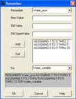
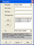
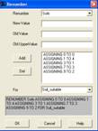
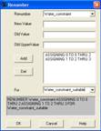
RENUMBER SLOPES
ASSIGNING 1 TO 20 THRU 65 ASSIGNING 5 TO 10 THRU 20 ASSIGNING 9 TO 0 THRU 10
FOR SLOPE_SUITABLE


![]()
Slope Map
Renumber Command
Slope_suitable Map
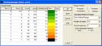
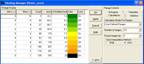
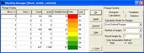
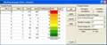
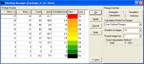
The
slope map is an example of a 2D grid map showing us values ranging from 0 to
65%. The slope map is renumbered so that
its values fall within the suitability range of 1 (poor suitability) to 9
(excellent suitability). The command
used in bold typeface indicates what values are assigned to the existing slope
values.
…very well presented and organized
COMPUTE
SLOPE_SUITABLE TIMES 6 FOR SLOPE_WEIGHTED …the weighting step is best reserved for when
you average the maps—can be done using the Analyze command (or in the Calculate
command sum using parentheses)
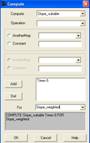

Compute
Command Slope_weighted Map
The
2D grid slope weighted map has values ranging from 6 to 54.
![]()
Page 13
2. Road Proximity Analysis
RENUMBER ROADS
ASSIGNING 0 TO 0 ASSIGNING 1 TO 1 THRU 43 FOR ROADS_SIMPLE
Roads Map Renumber
Command Roads_simple
Map
The
2D grid roads map with values of zero to 43 is renumbered to create the 2D grid
binary map (values of only zero or 1) of roads_simple. A zero value represents
all areas without a road while a 1 value on the roads_simple map represents a
road.
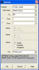
SPREAD ROADS_SIMPLE
TO 50 SIMPLY FOR ROADS_
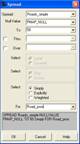
Spread
Command Roads_prox Map
The
“spread” command finds the shortest effective distance from all specified cells
(the roads on the roads_simple map) to a specified distance which in this case
was 50 cells, which allows us to look at the distance of all cells on the map
from the roads since the map is 25 x 25 cells.
The “simply” option measures the distance from the feature cell, the
roads, starting at a value of 1. The
values on the roads_prox map range from 0 to 10.7 cells from the road. A 0 value (black color on the map) represents
an actual road.
![]()
Page 14
RENUMBER
Renumber
Command Road_suitable Map
The
road_prox map is renumbered to create the 2D grid road_suitable map with values
ranging from 1 to 9.
COMPUTE
Compute
Command Road_prox_weighted Map
The
road_suitable map is multiplied by 2 to create the 2D grid road_prox_weighted
map. The values on this map range from 2
to 18. Red colors on the map represent
higher values.
![]()
Page 15
3. Water Proximity
Analysis
RENUMBER WATER
ASSIGNING 0 TO 0 ASSIGNING 1 TO 1 THRU 8 FOR WATER_SIMPLE
Water Map Renumber
Command Water_simple
Map
The
2D grid water map, with values ranging from 0 to 8, is renumbered to create the
2D grid binary map of water_simple with values of 0 (dry land areas, grey
colors) and 1 (water areas, red colors) on the map.
SPREAD WATER_SIMPLE
NULLVALUE PMAP_NUL TO 50 SIMPLY FOR WATER_
Spread
Command Water_prox
Map
We
used the “spread” command to find all of the locations within a 50 cell
distance of the water features. By
specifying a value of 50 so that we will see the distance for all cells on the
map from the water features since the map is 25 x 25 cells in size. The “simply” option will tell us the
effective distance from the water features starting with a value of 1
cell. The values on the water_prox map
range from 0 to 10. Cells with a zero
value (black color on the map) are cells that actually contain a water feature
(i.e. stream, lake, etc.).
![]()
Page 16
RENUMBER WATER_
Renumber
Command Water_suitable Map
The
2D grid water_suitable map shows us values ranging from 1 to 9. Red colors represent higher values.
COMPUTE WATER_SUITABLE
TIMES 4 FOR WEIGHTED_WATER_SUITABLE
Compute
Command Weighted_water_suitable Map
The
weighted_water_suitable map shows us values ranging from 4 to 36, with the red
colors on the map representing higher values.
![]()
Page 17
4, Road Visibility Analysis
RADIATE ROADS_SIMPLE
OVER ELEVATION TO 100 AT 1 NULLVALUE 0 COMPLETELY FOR
![]()
Roads_simple Map
Radiate Command Road_visibility Map
We
“radiate” the 2D grid binary roads_simple map to create the road_visibility
viewshed map. This map identifies for
each cell how many total times that cell is seen from all of the road location
cells (the “completely” option). The
visibility is determined by using the elevation map. The values on the road_visibility map range
from 0 (dark green colors, areas not seen) to 75 (red colors on the map, areas
that are highly visible).
RENUMBER
Renumber
Command Road_visible_suitable Map
The
2D grid road_visible_suitable map shows us values ranging from 1 (dark green
areas, lowest suitability) to 9 (red areas with the highest suitability).
![]()
Page 18
COMPUTE
Compute
Command
Road_visible_weighted Map
The
2D grid road_visible_weighted map shows us values ranging from 1 to 9, the same
values as on the road_visible_suitable map.
Since we multiplied the road_visible_suitable map by 1, no additional
weight factor is being assigned to this map.
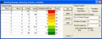
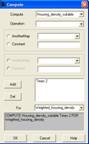
5. Housing Density Analysis
SCAN HOUSING TOTAL
IGNORE 0,0 WITHIN 3 SQUARE FOR HOUSING_DENSITY
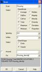
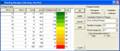
Housing Map Scan Command Housing_density Map
The
2D grid housing map with values ranging from 0 (no houses) to 5 (5 houses per
cell) is “scanned” to find the housing density.
Scan summarizes the values that occur within the vicinity of each
cell. We specify a distance of 3 cells
since we are interested in how many houses are within 3 cells of each cell on
the map. The “total” option replaces the
existing cell values with the sum of the cell values included in the scan. The housing density map shows us values of 0
(red colored areas, no houses, low density) to 30 (dark green areas with a high
housing density).
![]()
Page 19
RENUMBER
HOUSING_DENSITY ASSIGNING 1 TO 12 THRU 30 ASSIGNING 3 TO 6 THRU 12 ASSIGNING 7
TO 3 THRU 6 ASSIGNING 9 TO 0 THRU 3 FOR HOUSING_DENSITY_SUITABLE
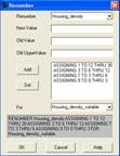
Renumber
Command
Housing_density_Suitable Map
The
housing_density_suitable map shows us values ranging from 1 (dark green areas, poor
suitability) to 9 (red colored areas, very high suitability).
COMPUTE
HOUSING_DENSITY_SUITABLE TIMES 2 FOR HOUSING_DENSITY_WEIGHTED
Compute
Command Housing_density_weighted Map
The
2D housing_density_weighted map shows us values ranging from 2 (dark green
areas, poor suitability) to 18 (red colored areas, high suitability).
![]() Page 20
Page 20
6. Soils Analysis
RENUMBER SOILS
ASSIGNING 0 TO 0 ASSIGNING 1 TO 4 ASSIGNING 3 TO 1 ASSIGNING 7 TO 3 ASSIGNING 9
TO 2 FOR SOIL_SUITABLE
Soils Map Renumber Command Soil_suitable Map
The
2D grid soils map with values ranging from 0 to 4 is renumbered to produce the soil_suitable
map with values ranging from 0 (grey areas on map with no soils) to 9 (red
colored areas with highly suitable soils).
COMPUTE SOIL_SUITABLE
TIMES 8 FOR WEIGHTED_SOIL_SUITABLE
Compute
Command Weighted_soil_suitable
Map
The
weighted_soil_suitable map has values ranging from 0 (grey areas with no soils)
to 72 (red colored areas with highly suitable soils.
![]()
Page 21
7. Steepness Constraint
RENUMBER SLOPE
ASSIGNING 1 TO 0 THRU 50 ASSIGNING 0 TO 50 THRU 65 FOR STEEPNESS_CONSTRAINT
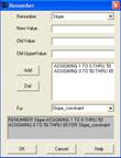
Slope Map Renumber
Command
Steepness_constraint Map
The
2D grid slope map with values of 0 to 65% is renumbered to create a 2D grid
binary steepness_constraint map. The
grey colored areas with a 0 value represent those areas where the slope is too
steep (greater than 50%) due to a county legal constraint. The red colored areas with a value of 1 are
areas with a slope less than 50% and it’s OK to build a landfill in these
areas.
8. Water Constraint
SPREAD WATER_SIMPLE
NULLVALUE PMAP_NULL TO 2 SIMPLY FOR WATER_CONSTRAINT

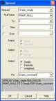
Water_simple Map Spread Command
Water_constraint Map
The
“spread” command is used to create a 1 cell wide buffer around all of the water
features. The water_constraint map shows
us values ranging from 0 (black colored areas, actual water features) to 3
(dark green areas that are 2 or more cells away from a water feature. The red colored areas with a value of 1
represent a 1 cell buffer in which a landfill cannot be located due to legal
constraints.
![]()
Page 22
RENUMBER
WATER_CONSTRAINT ASSIGNING 0 TO 0 THRU 2 ASSIGNING 1 TO 2 THRU 3 FOR
WATER_CONSTRAINT_SUITABLE
Renumber
Command Water_constraint_suitable Map
The
water_constraint map is renumbered to create a 2D grid binary map of
water_constraint_suitable with values of 0 (grey colored areas where it’s
illegal to build a landfill) and 1 (red colored areas where it is OK to build a
landfill).
9. Total Suitability
Maps
COMPUTE
SLOPE_WEIGHTED
…use parentheses in Calculate for weighting
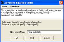
Compute Command
Total_suitability Map
The
total_suitability map shows us the suitability values ranging from 55 (dark
green areas, low suitability) to 183 (red colored areas on the map with high
suitability). This map is the result of
adding the 6 weighted suitability maps generated in sections 1 through 6 of the
Appendix.
![]()
Page 23
COMPUTE
TOTAL_SUITABILITY DIVIDEDBY 6 FOR AVERAGE_SUITABILITY
Compute
Command Average_suitability Map
The
total_suitability map is divided by 6 to produce the average_suitability
map. We divide by 6 since we used a
total of 6 different weighted suitability maps to find the
total_suitability. The
average_suitability map has values ranging from 9 (dark green areas with a low
suitability) to a 33 (red colored areas with a high suitability).
10. Final Suitable
Landfill Locations
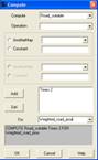
COMPUTE
AVERAGE_SUITABILITY TIMES WATER_CONSTRAINT_SUITABLE TIMES SLOPE_CONSTRAINT FOR
GARBAGE_R_US_SITES
Average_suitability
Map


Water_constraint Map Compute Command Garbage_R_Us_Sites
Steepness_constraint
Map
![]()
Page 24
When
we multiply the 3 maps shown above together, the 0 values on the constraint
maps (the grey colored areas) when multiplied with the average_suitability map
results in zero values on the final Garbage_R_Us_Sites map (the areas colored
in black). The values on the
Garbage_R_Us_Sites map range from 0 (black colored areas where it’s impossible
to build due to legal constraints or is physically impossible) to 30 (red
colored areas where it’s highly suitable to build a landfill).
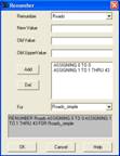
RENUMBER
GARBAGE_R_US_SITES ASSIGNING 0 TO 0 ASSIGNING 1 TO 1 THRU 9 ASSIGNING 3 TO 9
THRU 15 ASSIGNING 5 TO 15 THRU 21 ASSIGNING 7 TO 21 THRU 27 ASSIGNING 9 TO 27
THRU 30 FOR GARBAGE_R_US_SUITABLE
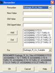
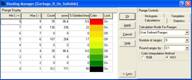
Renumber
Command Garbage_R_Us_Suitable Map
We
did a renumber on the Garbage_R_Us_Sites map so that the values would fall into
our suitability range of 0 (illegal, impossible to build black colored areas on
the map) to 9 (red colored areas where it is highly suitable to build a new
landfill based on our analysis).
RENUMBER
GARBAGE_R_US_SUITABLE ASSIGNING 0 TO 0 THRU 7 ASSIGNING 1 TO 7 THRU 9 FOR
GARBAGE_R_US_MOSTSUIT
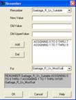
Renumber
Command Garbage_R_Us_Mostsuit Map
We
renumber the Garbage_R_Us_Suitable map to create a binary map that shows us to
see the areas with the highest suitabilities of values 7 to 9 being assigned a
value of 1 (red colors on the binary map) and areas with a suitability value of
7 or less are assigned a value of 0 (grey colored areas).
The
red colored areas on this map represent 422 acres of the site (27% of the total
area) which has a high suitability rating ( a value of 7 to 9 on the
Garbage_R_Us_Suitable Map).
![]()
Page 25
CLUMP
GARBAGE_R_US_SUITABLE AT 1 DIAGONALLY FOR GARBAGE_R_US_SUITABLE_AREAS

Clump Command Garbage_R_Us_Suitable_Areas
The
“clump” command allows us to uniquely identify groups of cells separately that
are geographically separated on the map.
This information is useful for us so we can see how much area (acres)
each group of connected cells has. The
map shows us that there are a total of 34 separate areas on the map. Areas numbered 5, 16, 19, 21, 22, 24 33, and
34 on the map are the ones with the highest suitability rating (these are the
red colored areas on the map).
COMPUTE
GARBAGE_R_US_SUITABLE_AREAS TIMES GARBAGE_R_US_MOSTSUIT FOR
GARBAGE_R_US_SITEAREAS
Compute
Command
Garbage_R_Us_Siteareas
These
2 maps are multiplied together so we can determine the number of acres for each
of the different sites (clumped areas with the same value) on the map. The black areas represent areas where there
is a legal constraint, it’s impossible to build in that location, or the
suitability rating is below a value of 7 on the Garbage_R_Us_Suitable map. We did this to get an idea of how many acres
of These black colored areas are a zero value on the Garbage_R_Us_Mostsuit map. Each value on this map represents a different
clumped area, so each number represents a different group of connected cells
with the same value.
The
largest area (red color) has an area of 227 acres while the 2nd
largest area is 49.4 acres at the lower left corner of the map in the light
green color.
![]()
Page 26
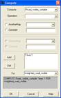
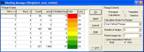
11. Average
Suitability Rating for Districts
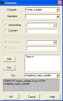
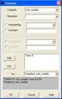
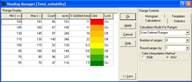
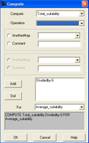
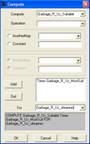
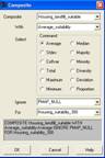
COMPOSITE DISTRICTS
WITH GARBAGE_R_US_SUITABLE AVERAGE IGNORE PMAP_NULL FOR
DISTRICTS_LANDFILL_SUITABLE
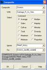

Districts Map Composite
Command
Garbage_R_Us_Suitable
Districts_landfill_suitable Map
Using
the “composite” command we are
able to summarize the values of one map (the districts map) with values of
another map (the Garbage_R_Us_Sites map) for each location on both maps. Composite gives us an average suitability
rating for each of the 7 districts.
District 1 had the lowest average suitability rating with a value
of 0 (upper left corner of the map where
there is a water feature) while District 6 in the lower right corner of the map
had the highest average suitability with a value of 4.78
![]()
Page 27
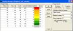
12.Housing Rating
Within 300 meters
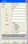
SPREAD HOUSING
NULLVALUE PMAP_NULL TO 4 WEIGHTED FOR HOUSING_LANDFILL_SUITABLE
…calculates for more than 300m—works but better
if you had used Scan around.

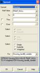
Housing Map Spread Command
Housing_landfill_suitable Map
The
housing map is “spread” to a distance of 4 cells, one more cell than we are
interested in to make sure that we don’t get only a partial value for a cell,
to determine the radius (or buffer) of cells around each housing location. The values on the housing_landfill_suitable
map range from 0 (dark green color meaning there is a house in that location)
to a 5 (red colored areas that indicate that there are no houses present in
that location). The “weighted” option
will apply a weight factor so that a cell with more houses will receive a
higher value than a cell with fewer houses near it.
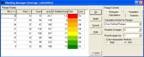
COMPOSITE
HOUSING_LANDFILL_SUITABLE WITH AVERAGE_SUITABILITY AVERAGE IGNORE PMAP_NULL FOR
HOUSING_SUITABILITY_300
Composite
Command Housing_suitability_300 Map
The
“composite” command was used to find the average suitability for each of the
houses within a 3 cell radius of the houses.
The housing_suitability_300 map shows us values ranging from 5.08 to
5.81, meaning that all of the houses are in areas of fairly high suitability
(on a scale of 0 being non-suitable to 9 being the most suitable).
![]()
Page 28