 Lab Assignment Guidelines
<click here> for a printer-friendly
version of the guidelines (.pdf)
Guidelines for Preparing and
Submitting Homework Assignments
Homework assignments use course software to address a series
of questions that illustrate and demonstrate
A high degree of professionalism in preparing your lab reports is expected. Generally speaking…
-
an A grade on the
labs requires work beyond the basic question
-
a B grade has a
good answer to the question, demonstrates an understanding of the basic
material and is well organized and presented
-
a C and lower
grades indicate incorrect answers and/or less than expected demonstration of
understanding, organization or presentation.
The lab assignments are worth 50 points each and
represent nearly half of your grade. In
addition, student teams will complete a mini-
Submitting
Lab Assignments: Store your completed exercises as Word
documents (.doc) in Web Layout View
and place in the class BlackBoard Dropbox and then email a note that you have
submitted it to the instructor. Do
not worry about page breaks or other printer formatting as all exchange of
the labs will be in electronic form. Grading will use the “Track changes”
tool in Word to grade, make comments then return the document.
Homework exercises will be
completed in two or three member teams.
To help us keep track, please name your homework files with the exercise
number followed by the team member names separated by an underscore (e.g., Exercise0_Smith_Jones_Brown.doc). The phrase “_graded” will be added when it is
graded and returned to each of the members on the team (e.g.,
Exercise0_Smith_Jones_Brown_graded.doc).
Homework assignments are expected
by the next class meeting but absolutely due by 5:00pm on the second
Friday following class (two extra days to complete if needed; send the
instructor an email if extra time is needed).
This allows an opportunity to discuss concerns during office hours and
after class on Thursday if you have difficulties in completing an
assignment. In addition, the class
Unexcused late homework
assignments without prior notification receive a maximum possible of 45 points
(10% penalty) if turned in prior to the next class meeting, and will not be
accepted (0 points) if more than one week late.
__________________________________
Example Question and Response: An example question and response is shown below. It illustrates a very good response (B+) addressing the basic question in a clear and concise manner. Outstanding responses (A+) usually go beyond the minimal bounds of a question by expanding the answer to include information from the readings and/or your own thoughts.
For example,
an interesting extension to the example question would be…
1)
Capturing
vertical 3D views of both displays (use the “Rotate” button to place the view
point directly down on the plot) then describe/explain the differences in the
“induced” 2-D plots and the vertical views of the 3-D surface.
2)
Or you might
investigate the Shading Manager controls on your own and generate displays with
different “contour” color assignments and discuss the visual impact of the
changes.
…however Exercise #0 will not
be graded.
__________________________________
 Exercise #0 — Displaying Map Surfaces (MapCalc)
Name: _____<enter name >_____
Date: _____<enter date>______
Email Address: __<insert response>___
Degree Program: __<insert response>___
Department: __<insert response>___
Professional Interests: __<insert response>___
Course Goals: __<insert response>___
General Computer Proficiency/Experience: __<insert response>___
Math/Stat Proficiency/Experience: __<insert response>___
Note: this Word document is in “Web Layout” format (from the
main menu, select View à Web Layout to verify).
Instructions and questions for your response are in blue 10-point
type. Yellow highlighted
areas are for your answers; just highlight and begin typing. When you enter
your responses, they will automatically be in black 12-point type. Grading notes
will be made in Red 12-point type when electronically returned to you. The exercise document will never be printed
as it saves trees, formatting headaches on your part and grading headaches on
the instructor’s part ...it’s a step toward your generation’s “paperless
society.”
Access the MapCalc system using the
TUTOR25 database as described by the instructor.
Use the following procedures to
generate a 3D display of the Elevation map:
ü From the Main Menu select Windowà Elevation
ü Press the 3-D Toggle view button to display the
elevation surface as a 3D plot
ü Press the Layer Mesh button to superimpose the grid
lines on the plot
ü Press the Use cells button to toggle between lattice
and grid displays of the elevation data.
Question 1. Screen capture and paste 3D” lattice” and “grid” displays of the Elevation map below (be sure to include a title and caption for each of the figures).
Insert figures…
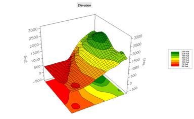
Figure 1-1. 3D Lattice Display. Note the smooth
appearance of the plot that “stretches” the grid pattern by pushing up the
intersections of the grid lines.
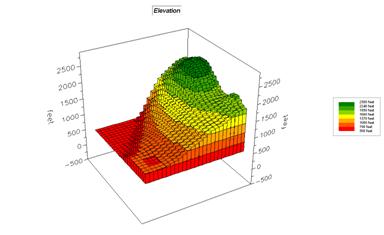
Figure 1-2. 3D Grid Display. Note the chunky appearance of the plot pushes
up the “pillars” representing each grid cell border.
In your own words describe the major differences between “lattice” and “grid” displays of mapped data?
Insert your answer…
A 3D representation of lattice data is analogous to draping a fishnet over the map values. Each intersection is raised to a relative height based on the value at the location. A perspective drawing of the fishnet is achieved by making the lengths of the lines correspond to the relative differences in the stored map values. Note the pronounced diamond shapes in the steep areas, while the flat areas form smaller square-like shapes.
The three-dimensional effect in a 3D Grid map is achieved by “extruding” each cell to a height based on its stored map value. Hidden line removal retains only the visible faces of the “bars” depending on viewer position and the spatial patterns in the data.
Also it is important to note that the “lattice” and “grid” 3-D displays in figure 1-1 and figure 1-2 use the same data layer that is stored as 25 columns by 25 rows (625 cells). The differences in appearance are due to display technique, not changes in the underlying data.
__________________________________