|
Beyond
Mapping IV Topic 2
– Extending Effective Distance Procedures (Further Reading) |
GIS Modeling book |
Just
How Crooked Are Things? — discusses distance-related metrics for
assessing crookedness (November 2012)
Extending
Information into No-Data Areas — describes a technique for
“filling-in” information from surrounding data into no-data locations (July 2011)
In Search of the Elusive Image
— describes extended geo-query techniques for accessing images containing
a location of interest (July 2013)
<Click here> for a printer-friendly version of this topic (.pdf).
(Back
to the Table of Contents)
______________________________
Just
How Crooked Are Things?
(GeoWorld,
November 2012)
In a heated presidential election month this seems to be an apt title
as things appear to be twisted and contorted from all directions. Politics aside and from a down to earth
perspective, how might one measure just how spatially crooked things are? My benchmark for one of the most crooked
roads is Lombard Street in San Francisco—it’s not only
crooked but devilishly steep. How might
you objectively measure its crookedness?
What are the spatial characteristics?
Is Lombard Street more crooked than the eastern side of Colorado’s
Independence Pass connecting Aspen and Leadville?
Webster’s Dictionary defines crooked as “not straight” but there is a
lot more to it from a technical perspective.
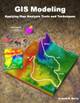
For example, consider the two paths along a road network shown in figure
1. A simple crooked comparison
characteristic could compare the “crow flies” distance (straight line) to the
“crow walks” distance (along the road).
The straight line distance is easily measured using a ruler or
calculated using the Pythagorean Theorem.
The on-road distance can be manually assessed by measuring the overall
length as a series of “tick marks” along the edge of a sheet of paper
successively shifted along the route. Or
in the modern age, simply ask Google Maps for the route’s distance.
The vector-based solution in Google Maps, like the manual technique,
sums all of the line segments lengths comprising the route. Similarly, a grid-based solution counts all
of the cells forming the route and multiplies by an adjusted cell length that
accounts for orthogonal and diagonal movements along the sawtooth representation. In both instances, a Diversion Ratio
can be calculated by dividing the crow walking distance (crooked) by the crow
flying distance (straight) for an overall measurement of the path’s diversion
from a straight line.
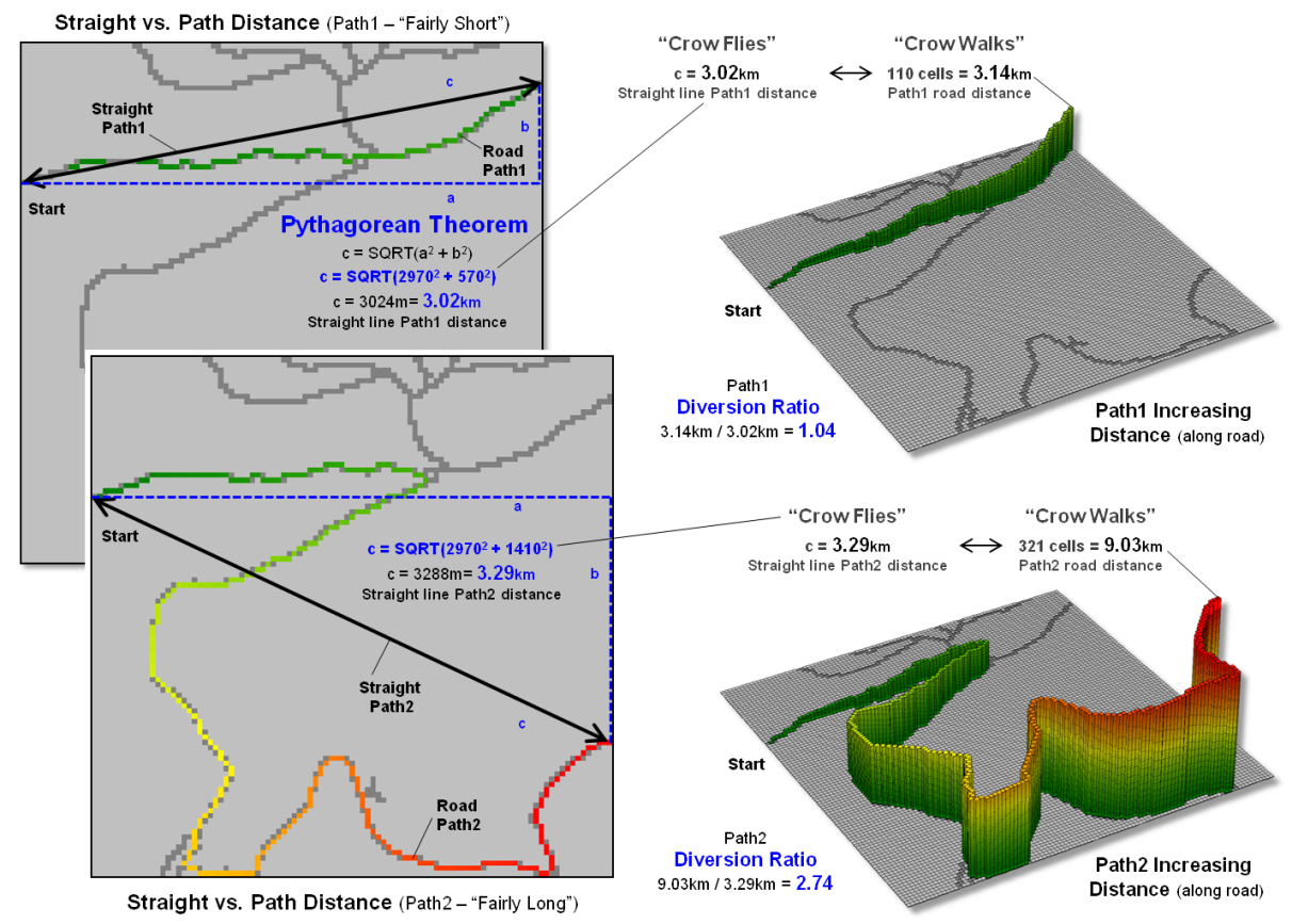
Figure 1. A Diversion Ratio
compares a route’s actual path distance to its straight line distance.
As shown in the figure the diversion ratio for Path1 is 3.14km / 3.02km
= 1.04 indicating that the road distance is just a little longer than the
straight line distance. For Path2, the
ratio is 9.03km / 3.29km = 2.74 indicating that the Path2 is more than two and
a half times longer than its straight line.
Based on crookedness being simply “not straight,” Path2 is much more
crooked.
Figure 2 depicts an extension of the diversion ratio to the entire road
network. The on-road distance from a
starting location is calculated to identify a crow’s walking distance to each
road location (employing Spatial Analyst’s Cost Distance tool for the
Esri-proficient among us). A straight
line proximity surface of a crow’s flying distance from the start is generated
for all locations in a study area (Euclidean Distance tool) and then isolated
for just the road locations. Dividing
the two maps calculates the diversion ratio for every road cell.
The ratio for the farthest away road location is 321 cells /117 cells =
2.7, essentially the same value as computed using the Pythagorean Theorem for
the straight line distance. Use of the
straight line proximity surface is far more efficient than repeatedly
evaluating the Pythagorean Theorem, particularly when considering typical
project areas with thousands upon thousands of road cells.
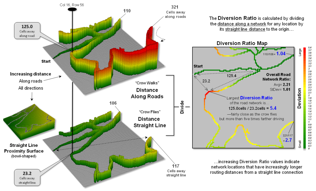
Figure 2. A Diversion Ratio Map
identifies the comparison of path versus straight line distances for every
location along a route.
In addition, the spatially disaggregated approach carries far more
information about the crookedness of the roads in the area. For example, the largest diversion ratio for
the road network is 5.4—crow walking distance nearly five and a half times that
of crow flying distance. The average
ratio for the entire network is 2.21 indicating a lot of overall diversion from
straight line connection throughout the set of roads. Summaries for specific path segments are
easily isolated from the overall Diversion Ratio Map— compute once, summarize
many. For example, the US Forest Service
could calculate a Diversion Ratio Map for each national forest’s road system
and then simply “pluck-off” crookedness information for portions as needed in
harvest or emergency-response planning.
The Deviation Index shown in figure 3 takes an entirely
different view of crookedness. It
compares the deviation from a straight line connecting a path’s end points for
each location along the actual route.
The result is a measure of the “deflection” of the route as the
perpendicular distance from the centerline.
If a route is perfectly straight it will align with the centerline and
contain no deflections (all deviation values= 0). Larger and larger deviation values along a
route indicate an increasingly non-straight path.
The left side of figure 3 shows the centerline proximity for Paths 1
and 2. Note the small deviation values
(green tones) for Path 1 confirming that is generally close to the
centerline. This confirms that it is
much straighter than Path 2 with a lot of deviation values greater than 30
cells away (red tones). The average
deflection (overall Deviation Index) is just 3.9 cells for Path1 and 26.0 cells
for Path2.
Figure 3. A Deviation Index
identifies for every location along a route the deflection from a path’s
centerline.
But crookedness seems more than just longer diverted routing or
deviation from a centerline. It could be
that a path simply makes a big swing away from the crow’s beeline flight—a
smooth curve not a crooked, sinuous path.
Nor is the essence of crookedness simply counting the number of times
that a path crosses its direct route.
Both paths in the examples cross the centerline just once but they are
obviously very different patterns.
Another technique might be to keep track of the above/below or
left/right deflections from the centerline.
The sign of the arithmetic sum would note which side contains the
majority of the deflections. The
magnitude of the sum would report how off-center (unbalanced) a route is. Or maybe a roving window technique could be
used to summarize the deflection angles as the window is moved along a route.
The bottom line (pun intended) is that spatial analysis is still in its
infancy. While non-spatial math/stat
procedures are well-developed and understood, quantitative analysis of mapped
data is very fertile turf for aspiring minds …any bright and inquiring grad
students out there up to the challenge?
_____________________________
Author’s
Note: For a related discussion of characterizing
the configuration of landscape features, see the online book Beyond Mapping I,
Topic 5: Assessing Variability, Shape, and Pattern of Map Features posted at www.innovativegis.com/basis/BeyondMapping_I/Topic5/.
__________________________________
Additional
discussion of distance, proximity, movement and related measurements in
-
Topic 25,
Calculating Effective Proximity
-
Topic 20,
Surface Flow Modeling
-
Topic 19,
Routing and Optimal Paths
-
Topic 17,
Applying Surface Analysis
-
Topic 15,
Deriving and Using Visual Exposure Maps
-
Topic 14,
Deriving and Using Travel-Time Maps
-
Topic 13,
Creating Variable-Width Buffers
-
Topic 6,
Analyzing In-Store Shopping Patterns
-
Topic 5,
Analyzing Accumulation Surfaces
Extending Information into No-Data Areas
(GeoWorld, July
2011)
I am increasingly intrigued by wildfire modeling. For a spatial analysis enthusiast, it has it
all— headlines grabbing impact, real-world threats to life and property, action
hero allure, as well as a complex mix of geographically dependent “driving
variables” (fuels, weather and topography) and extremely challenging spatial
analytics.
However with all of their sophistication, most wildfire models tend to
struggle with some very practical spatial considerations. For example, figure 1 identifies an extension
that “smoothes” the salt and pepper pattern of the individual estimates of
flame length for individual 30m cells (left side) into a more continuous
surface (right side). This is done for
more than cartographic aesthetics as surrounding fire behavior conditions are
believed to be important. It makes sense
that an isolated location with predicted high flame length conditions adjacent
to much lower values is presumed to be less likely to attain the high value
than one surrounded by similarly high flame length values. Also the mixed-pixel and uncertainty effects
at the 30m spatial resolution suggest using a less myopic perspective.
The top right portion of the figure shows the result of a
simple-average 5-cell smoothing window (150m radius) while the lower inset
shows results of a 10-cell reach (300m).
Wildfire professionals seem to vary in their expert opinion (often in
heated debate—yes, pun intended) of the amount and type of smoothing required,
but invariably they seem to agree that none (raw data) is too little and a
10-cell reach is too much. The most
appropriate reach and the type of smoothing to use will likely keep fire scientists
busy for a decade or more. In the
interim, expert opinion prevails.
An even more troubling limitation of traditional wildfire models is
depicted as the “white region” in figure 1 representing urban areas as
“no-data,” meaning they are areas of “no wildland fuel data” and cannot be
simulated with a wildfire model. The
fuel types and conditions within an urban setting form extremely complex and
variable arrangements of non-burnable to highly flammable conditions. Hence, the wildfire models must ignore urban
areas by assigning no-data to these extremely difficult conditions.
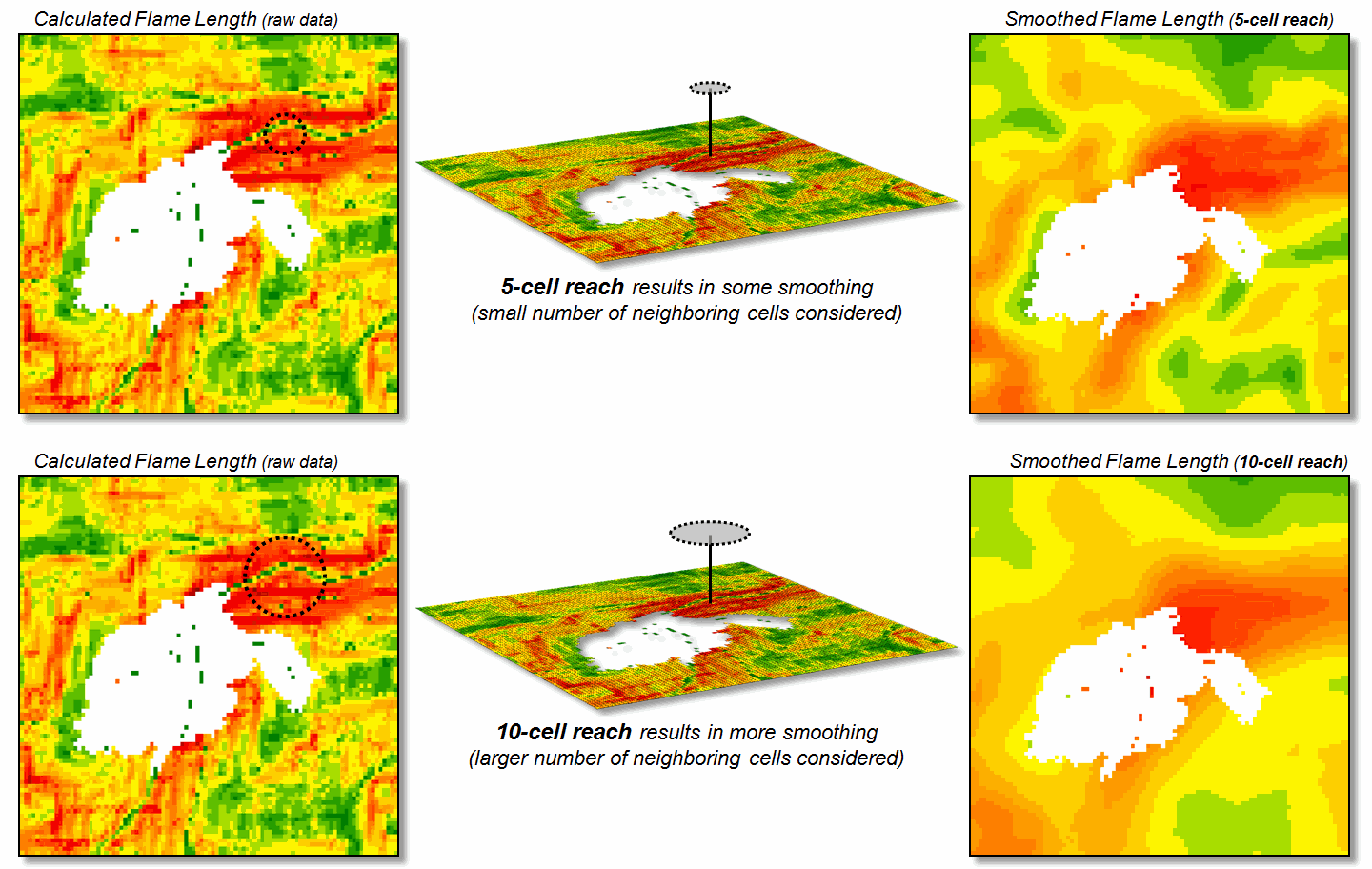
Figure 1. Raw Flame Length values
are smoothed to identify the average calculated lengths within a specified
distance of each map location— from point-specific condition to a localized
condition that incorporates the surrounding information (smoothing).
However all too often, wildfires ignore this artificial boundary and
move into the urban fringe. Modeling the
relative venerability and potential impacts within the “no data” area is a
critical and practical reality.
Figure 2 shows the first step in extending wildfire conditions into an
urban area. A proximity map from the
urban edge is created and then divided into a series of rings. In this example, a 180m overall reach into
the urban “no-data” area uses three 2-cell rings.
A roving window of 4-cells is used to average the neighboring flame
lengths for each location within the First Ring and these data are added to the
original data. The result is “oozing”
the flame lengths a little bit into the urban area. In turn, the Second Ring’s average is
computed and added to the Original plus First Ring data to extend the flame
length data a little bit more. The
process is repeated for the Third Ring to “ooze” the original data the full 180
meters (6-cell) into the urban area (see figure 3).
It is important to note that this procedure is not estimating flame
lengths at each urban location, but a first-cut at extending the average flame
length information into the urban fringe based on the nearby wildfire behavior
conditions. Coupling this information with
a response function implies greater loss of property where the nearby flame
lengths are greater.
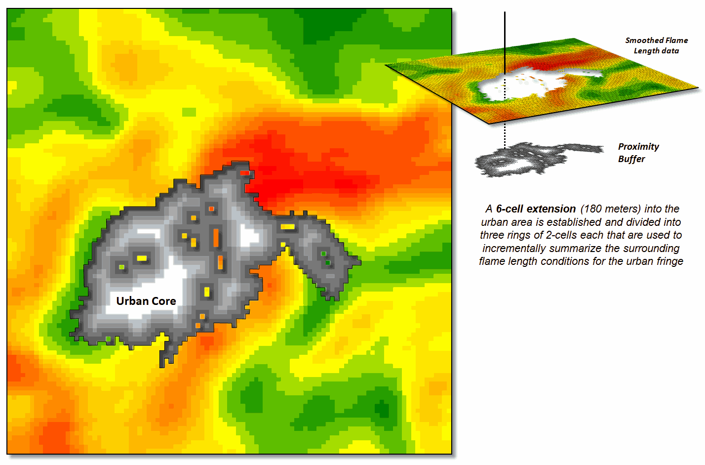
Figure 2. Proximity rings
extending into urban areas are calculated and used to incrementally “step” the
flame length information into the urban area.
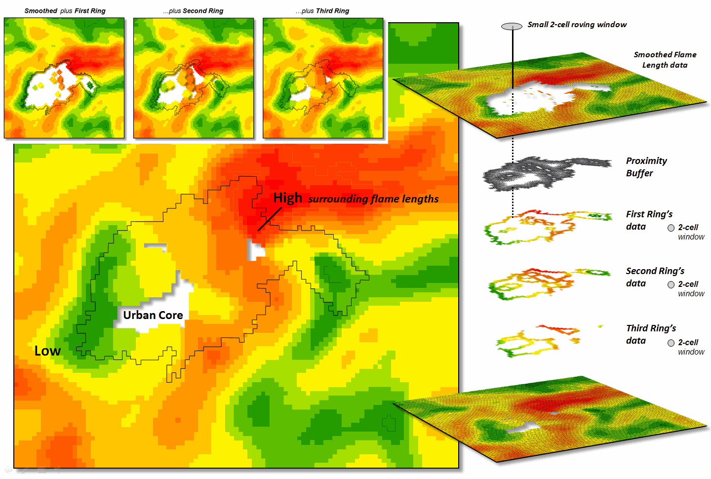
Figure 3. The original smoothed
flame length information is added to the First Ring’s data, and then
sequentially to the Second Ring’s and Third Ring’s data for a final result that
extends the flame length information into the urban area.
Locations in red identify generally high neighboring flame lengths,
while green identify generally low locations—a first-cut at the relative
wildfire threat within the urban fringe.
What is novel in this procedure is the iterative use of nested rings to
propagate the information—“oozing” the data into the urban area instead of one
large “gulp.” If a single large roving
window (e.g., a 10-cell radius) were used for the full 180 meter reach
inconsistencies arise. The large window
produces far too much smoothing at the urban outer edge and has too little information
at the inner edge as most of the window will contain “no-data.”
The ability to “iteratively ooze” the information into an area
step-by-step keeps the data bites small and localized, similar to the brush
strokes of an artist.
_____________________________
Author’s
Note: For more discussion of
roving windows concepts, see the online book, Beyond Modeling III, Topic
26, Assessing Spatially-Defined Neighborhoods at www.innovativegis.com/Basis/MapAnalysis/Default.htm.
In Search of the Elusive Image
(GeoWorld, July
2013)
Last year National Geographic reported that nearly a billion photos
were taken in the U.S. alone and that nearly half were captured using camera
phones. Combine this with work-related
imaging for public and private organizations and the number becomes staggering. So how can you find the couple of photos that
image a specific location in the mountainous digital haystack?
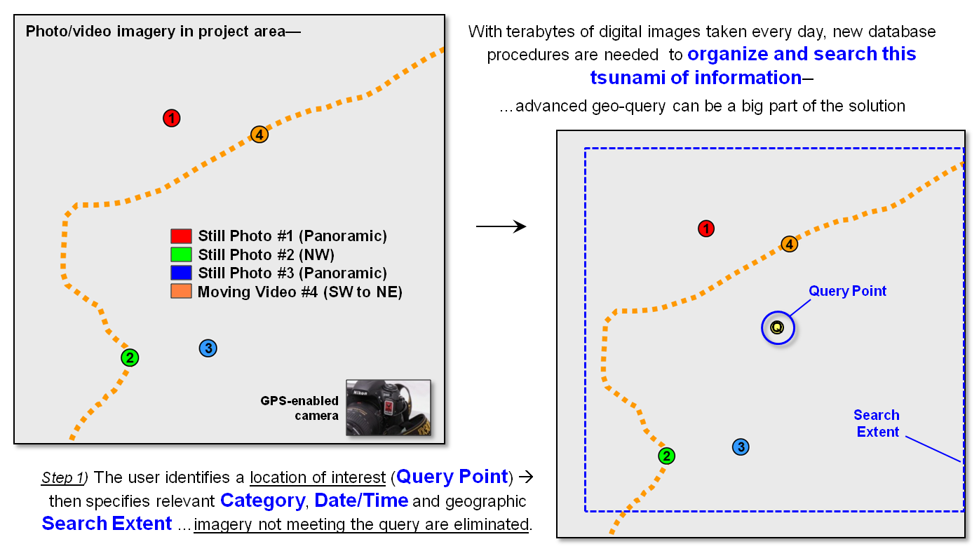
Figure 1. Geo-tagged photos and
streaming video extend traditional database category and date/time searches for
relevant imagery.
For the highly organized folks, a cryptic description and file folder
scheme can be used to organize logical groupings of photos. However, the most frequently used automated
search technique uses the date/time stamp in the header of every digital
photo. And if a GPS-enabled camera was
used, the location of an image can further refine the search. For most of us the basic techniques of Category,
Date/Time and Vicinity are sufficient for managing and accessing
a relatively small number of vacation and family photos (step 1, figure
1).
However if you are a large company or agency routinely capturing
terabytes of still photos and moving videos, searching by category, date/time
and earth position merely reduces the mountain of imagery to thousands
possibilities that require human interpretation to complete the search. Chances are most of the candidate image
locations are behind a hill or the camera was pointed in the wrong direction to
have captured the point of interest.
Simply knowing that the image is “near” a location doesn’t mean it
“sees” it.
Figure 2 outlines an approach that takes automated geo-searching a bit
farther (see author’s note 1). Step 2 in
the figure involves calculating the Viewshed from the query point
considering intervening terrain, cover type and the height of the camera. All of the potential images located outside
of the viewshed (grey areas) are not “visually connected” to the query point,
so the point of interest cannot appear in the image. These camera locations are eliminated.
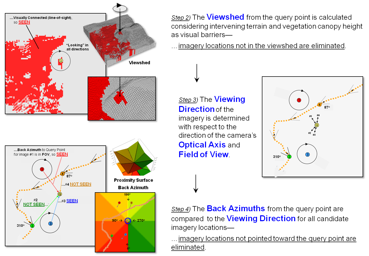
Figure 2. Viewshed Analysis
determines if a camera location can be seen from a location of interest and
Directional Alignment determines if the camera was pointed in the right
direction.
A third geo-query technique is a bit more involved and requires a
directionally-aware camera (step 3 in figure 2). While a lot of GPS-enabled cameras record the
position a photo was taken, few currently provide the direction/tilt/rotation
of the camera when an image is taken.
Specialized imaging devices, such as the three-axis gyrostabilizer mount used in aerial
photography, have been available for years to continuously
monitor/adjust a camera’s orientation.
However, pulling these bulky and expensive commercial instruments out of
the sky is an impractical solution for making general use cameras directionally
aware.
On the other hand, the gyroscope/accelerometers in
modern smartphones primarily used in animated games routinely measure
orientation, direction, angular motion and rotation of the device that can be
recorded with imagery as the technology advances. All that is needed is a couple of smart
programmers to corral these data into an app that will make tomorrow’s
smartphones even smarter and more aware of their environment to include where
they are looking, as well as where they are located. Add some wheels and a propeller for motion
and the smarty phone can jettison your pocket.
The final puzzle piece for fully aware imaging—lens geometry— has been
in place for years embedded in a digital photo’s header lines. The field of view (FOV) of a camera can be
thought of as a cone projected from the lens and centered on its optical
axis. Zooming-in changes the effective
focal length of the lens that in turn changes the cone’s angle. This results in a smaller FOV that records a
smaller area of the scene in front of a camera.
Exposure settings (aperture and shutter speed) control the depth of
field that determines the distance range that is in focus.
The last step in advanced geo-query for imagery containing a specified
location mathematically compares the direction and FOV of the optical cone to
the desired location’s position. A
complete solution for testing the alignment involves fairly complex solid
geometry calculations. However, a first
order planimetric solution is well within current map analysis toolbox capabilities.
A simple proximity surface from the specified location is derived and
then the azimuth for each grid location on the bowl-like surface is calculated
(step 4 in figure 2). This “back
azimuth” identifies the direction from each map location to the specified
location of interest. Camera locations
where the back azimuth is not within the FOV angle means the camera wasn’t
pointed in the right direction so they are eliminated.
In addition, the proximity value at a connected camera location indicates
how prominent the desired location is in the imaged scene. The different between the optical axis
direction and the back azimuth indicates the location’s centering in the image.
Figure 3 summarizes the advanced geo-query procedure. The user specifies the desired image
category, date/time interval and geographic search extent, and then “clicks” on
a location of interest. Steps 2, 3 and 4
are automatically performed to narrow down the terabytes of stored imagery to
those that are within the category/date/time/vicinity specifications, within
the viewshed of the location of interest and pointed toward the location of
interest. A hyperlinked list of photos
and streaming video segments is returned for further visual assessment and
interpretation.
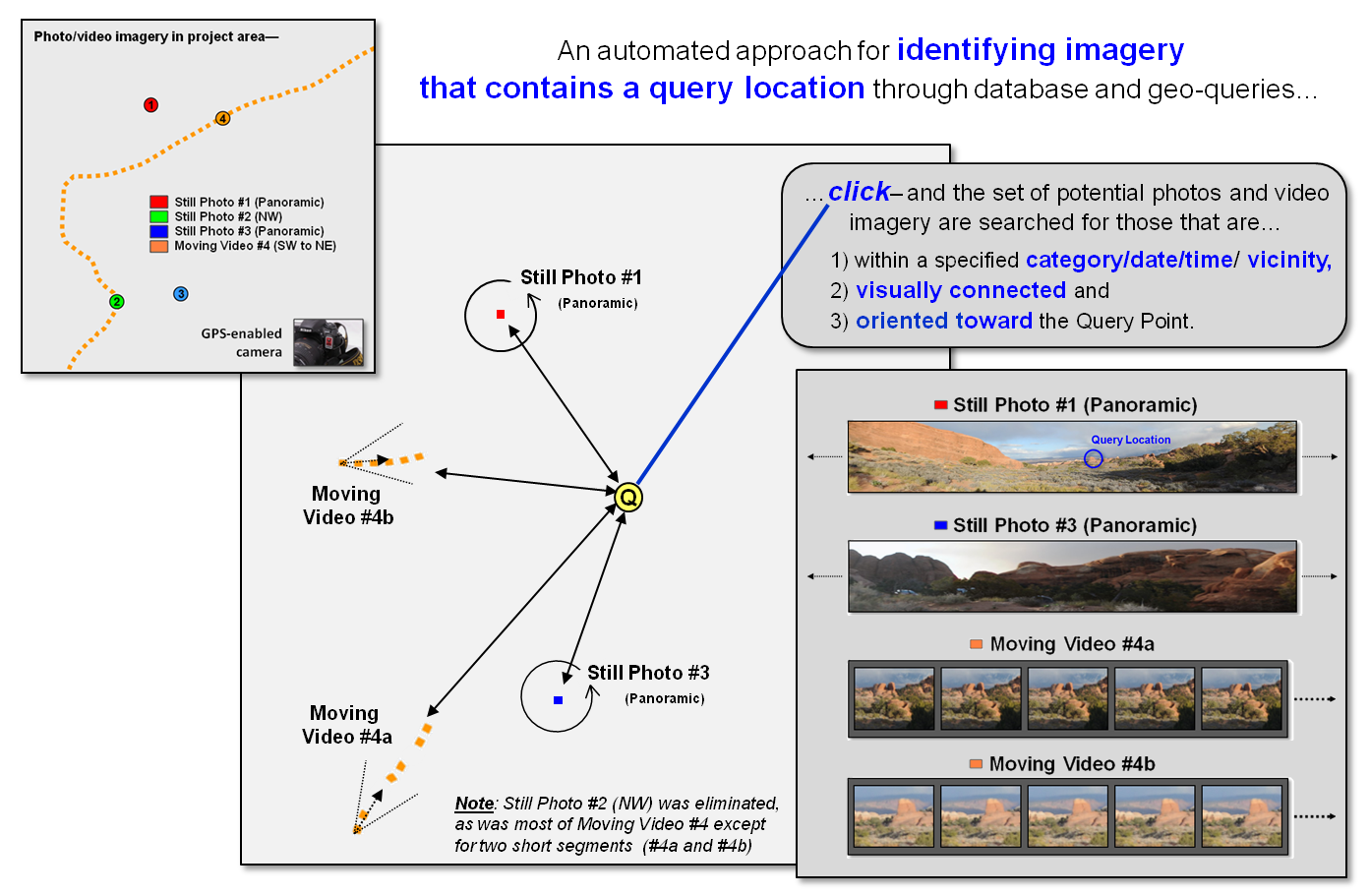
Figure 3. Advanced geo-query
automatically accesses relevant nearby imagery that is line-of-sight connected
and oriented toward a query point.
While full implementation of the automated processing approach awaits
smarter phones/cameras (and a couple of smart programmers), portions of the
approach (steps 1and 2) are in play today.
Simply eliminating all of the GPS-tagged images within a specified
distance of a desired location that are outside its viewshed will significantly
shrink the mountain of possibilities—tired analyst’s eyes will be forever
grateful.
_____________________________
Author’s Notes: 1) The advanced geo-query approach described
follows an early prototype technique developed for Red Hen Systems, Fort
Collins, Colorado.
(Back to the Table of Contents)