Beyond Mapping IV
|
GIS Modeling book |
Organizing
Geographic Space for Effective Analysis — an overview of data
organization for grid-based map analysis
Contour
Lines versus Color Gradients for Displaying Spatial Information — discusses
the similarities and differences between discrete contour line and continuous
gradient procedures for visualizing map surfaces
VtoR
and Back! — describes various techniques for converting between vector
and raster data types
Setting
a Place at the Table for Grid-based Data — describes the differences
between individual file and table storage approaches
<Click here>
for a printer-friendly version of this
topic (.pdf).
(Back to the Table of Contents)
______________________________
Organizing Geographic Space for
Effective Analysis
(GeoWorld, September 2012)
A basic familiarity of the two fundamental data types supporting geotechnology—vector and raster—is important for understanding map analysis procedures and capabilities (see author’s note). Vector data is closest to our manual mapping heritage and is familiar to most users as it characterizes geographic space as collection of discrete spatial objects (points, lines and polygons) that are easy to draw. Raster data, on the other hand, describes geographic space as a continuum of grid cell values (surfaces) that while easy to conceptualize, requires a computer to implement.
Generally speaking, vector data is best for traditional map display and geo-query—“where is what,” applications that identify existing conditions and characteristics, such as “where are the existing gas pipelines in Colorado” (a descriptive query of existing information). Raster data is best for advanced graphics and map analysis— “why, so what and what if” applications that analyze spatial relationships and patterns, such as “where is the best location for a new pipeline” (a prescriptive model deriving new information).
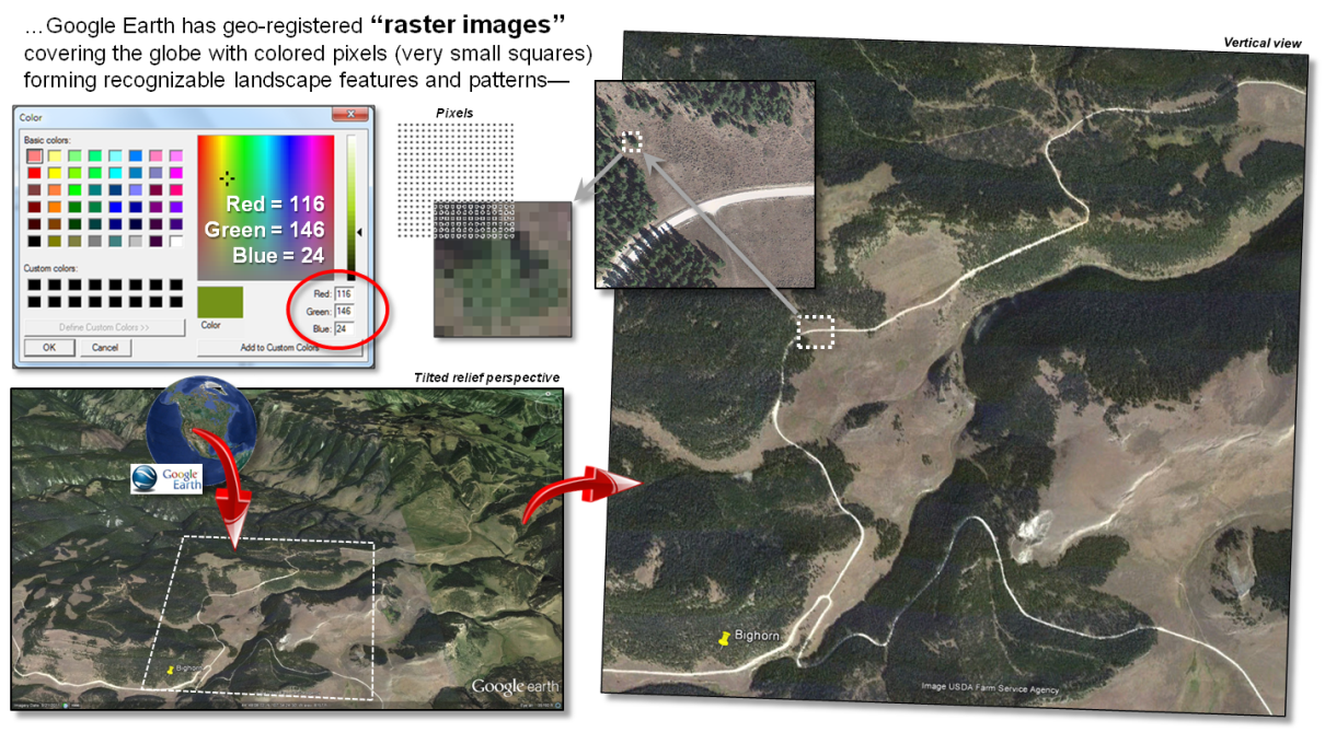
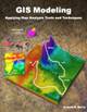
Figure 1. A
raster image is composed of thousands of numbers identifying different colors
for the “pixel” locations in a rectangular matrix supporting visual
interpretation.
Most vector applications involve the extension of manual mapping and inventory procedures that take advantage of modern computers’ storage, speed and Internet capabilities (better ways to do things). Raster applications, however, tend to involve entirely new paradigms and procedures for visualizing and analyzing mapped data that advances innovative science (entirely new ways to do things).
On the advanced graphics front, the lower-left portion of figure 1 depicts an interactive Google Earth display of an area in northern Wyoming’s Bighorn Mountains showing local roads superimposed on an aerial image draped over a 3D terrain perspective. The roads are stored in vector format as an interconnecting set of line features (vector). The aerial image and elevation relief are stored as numbers in geo-referenced matrices (raster).
The positions in a raster image matrix are referred to as “pixels,” short for picture elements. The value stored at each pixel corresponds to a displayed color as a combination of red, green and blue hues. For example, the green tone for some of the pixels portraying the individual tree in the figure is coded as red= 116, green= 146 and blue= 24. Your eye detects a greenish tone with more green than red and blue. In the tree’s shadow toward the northwest the red, green and blue levels are fairly equally low (dark grey). In a raster image the objective is to generate a visual graphic of a landscape for visual interpretation.
A raster grid is a different type of raster format where the values indicate characteristics or conditions at each location in the matrix designed for quantitative map analysis (spatial analysis and statistics). The elevation surface used to construct a tilted relief perspective in a Google Earth display is composed of thousands of matrix values indicating the undulating terrain gradient.
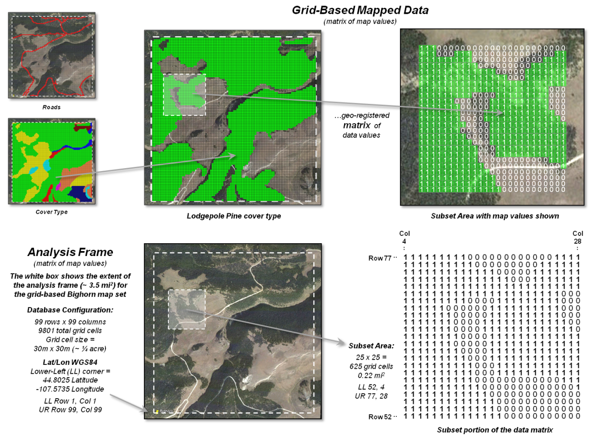
Figure 2. A raster grid contains a map values for each
“grid cell” identifying the characteristic/condition at that location
supporting quantitative analysis.
Figure 2 depicts a raster grid of the vegetation in the Bighorn area by assigning unique classification values to each of the cover types. The upper portion of the figure depicts isolating just the Lodepole Pine cover type by assigning 0 to all of the other cover types and displaying the stored matrix values for a small portion of the project area. While you see the assigned color in the grid map display (green in this example), keep in mind that the computer “sees” the stored matrix of map values.
The lower portion of the figure 2 identifies the underlying organizational structure of geo-registered map data. An “analysis frame” delineates the geographic extent of the area of interest and in the case of raster data the size of each pixel/grid element. In the example, the image pixel size for the visual backdrop is less than a foot comprising well over four million values and the grid cell size for analysis is 30 meters stored as a matrix with 99 columns and 99 rows totally nearly 10,000 individual cell locations.
For geo-referencing, the lower-left grid cell is identified as the matrix’s origin (column 1, row1) and is stored in decimal degrees of latitude and longitude along with other configuration parameters as a few header lines in the file containing the matrix of numbers. In most instances, the huge matrix of numbers is compressed to minimize storage but uncompressed on-the-fly for display and analytical processing.
Figure 3. A set of geo-registered map layers forms a
“map stack” organized as thousands upon thousands of numbers within a common
“analysis frame.”
Figure 3 illustrates a broader level of organization for grid-based data. Within this construct, each grid map layer in a geographically registered analysis frame forms a separate theme, such as roads, cover type, image and elevation. Each point, line and polygon map feature is identified as a grid cell grouping having a unique value stored in implied matrix charactering a discrete spatial variable. A surface gradient, on the other hand, is composed of fluctuating values that track the uninterrupted increases/decreases of a continuous spatial variable.
The entire set of grid layers available in a database is termed a map stack. In map analysis, the appropriate grid layers are retrieved, their vales map-ematically processed and the resulting matrix stored in the stack as a new layer— in the same manner as one solves an algebraic equation, except that the variables are entire grid maps composed of thousands upon thousands of geographically organized numbers.
The major advantages of grid-based maps are their inherently uncomplicated data structure and consistent parsing within a holistic characterization of geographic space—just the way computers and math/stat mindsets like it. No sets of irregular spatial objects scattered about an area that are assumed to be completely uniform within their interiors… rather, continuously defined spatial features and gradients that better align with geographic reality and, for the most part, with our traditional math/stat legacy.
The next section’s discussion builds on this point by extending grid maps and map analysis to “a universal key” for unlocking spatial relationships and patterns within standard database and quantitative analysis approaches and procedures.
_____________________________
Author’s Notes: For a more detailed discussion of vector and
raster data types and important considerations, see book III, Topic 1, “Data
Structure Implications” and book I, Topic 1, “Maps as Data” in the online book
Beyond Mapping Compilations Series posted at www.innovativegis.com/basis/MapAnalysis/.
Contour Lines versus Color
Gradients for Displaying Spatial Information
(GeoWorld, November 2011)
In mapping, there are historically three fundamental map features—points, lines and areas (also referred to as polygons or regions)—that partition space into discrete spatial objects (discontinuous). When assembled into a composite visualization, the set of individual objects are analogous to arranging the polygonal pieces in a jigsaw puzzle and then overlaying the point and line features to form a traditional map display. In paper and electronic form, each separate and distinct spatial object is stored, processed and displayed individually.
By definition line features are constructed by
connecting two or more data points. Contour lines are a form of
displaying information that have been used for many years and are a
particularly interesting case when displaying information in the computer
age. They represent a special type of
spatial object in that they connect data points of equal value. A contour
map is typically composed of a set of contour lines with intervening spaces
generally referred to as contour intervals.
In general usage, the word “line” in the term
“contour line” has been occasionally dropped, resulting in the ill-defined
terms of “contour” for an individual contour line and “contours” for a set of
contour lines or contour intervals depending on whether your focus is on the
lines or the intervening areas.
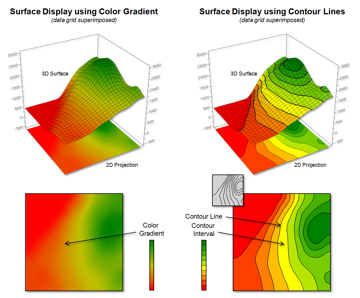
Figure 1. Surface displays using Contour Lines and
Color Gradient techniques.
The underlying concept is that contour lines are
lines that are separate and distinct spatial objects that connect data points
of equal value and are displayed as lines to convey this information to the
viewer. Historically these values
represented changes in elevation to generate a contour map of a landscape’s
undulating terrain, formally termed topographical relief.
Today, contour lines showing equal data values
at various data levels are used to represent a broad array of spatial data from
environmental factors (e.g., climatic temperature/pressure, air pollution
concentrations) to social factors (e.g., population density, crime rates) to
business intelligence (e.g., customer concentration, sales activity). Within these contexts, the traditional
mapping focus has been extended into the more general field of data
visualization.
With the advent of the computer age and the
associated increased processing power of the computer, a fourth type of
fundamental map feature has emerged—surfaces—an uninterrupted gradient (continuous).
This perspective views space as a continuously changing variable
analogous to a magnetic field without interruption of discrete spatial object
boundaries. In electronic form, a continuous surface is commonly stored
as two-dimensional matrix (x,y)
with a data value (z) at each grid location. These data are often
displayed as a 3-dimentional surface with the x,y-coordinates orienting the visualization plane in
space and the z-value determining the relative height above the plane.
In general, a 2-dimensional rendering of surface
data can be constructed two ways—using a continuous color gradient or by
generating a set of contour lines connecting points of equal data value
(see figure 1).
As shown in the figure, the color gradient
uses a continuum of colors to display the varying data across the surface. The contour line display, on the other hand,
utilizes lines to approximate the surface information.
Contour intervals can be filled with a color or can be displayed as a solid background (left-side of figure 1). For displays of contour lines, the lines convey the information to the view as a set of lines of constant values. The contour intervals do not have constant values as they depict a range values.
Figure 2 shows some of the visual differences in the two types of display approaches. The top portion of the figure depicts the positioning (Data Points) and storage of the spatial information (Data Values) that characterize surface data. A reference grid is established and the data points are positioned at specific x,y-locations within the reference grid. This arrangement is stored as a matrix of data values in a computer with a single value corresponding to each grid cell. Both contour lines and continuous color gradient displays use this basic data structure to store surface data.
Differences between the two approaches arise, however, in how the data is processed to create a display and, ultimately, how the information is displayed and visualized. Typically, color gradient displays are generated by assigning a color from a continuous spectrum to each grid cell based on the magnitude of the data value (lower left side of figure 2). For example, the 1843 value is assigned light green along the continuous red to green color spectrum. The color-fill procedure is repeated for all of the other grid spaces resulting in a continuous color gradient over an entire mapped area thereby characterizing the relative magnitudes of the surface values.
Contour line displays, on the other hand,
require specialized software to calculate lines of equal data value and, thus,
a visualization of a surface (right side of figure 2). Since the stored
data values in the matrix do not form adjoining data that are of a constant
data value, they cannot be directly connected as contour lines.
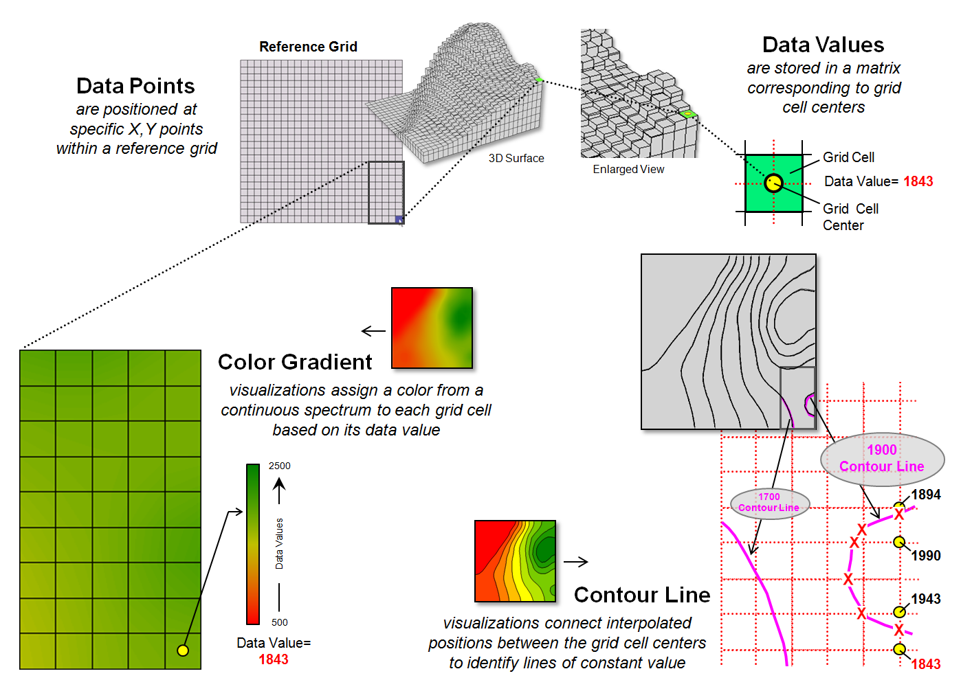
Figure 2. Procedures for creating surface displays
using Color Gradient and Contour Line techniques.
For example, the derivation of a “1900 value”
contour line involves interpolating the implied data point locations for the
line from the centers of the actual gridded data as shown in the figure. The two data values of 1843 to 1943 in the
extreme lower right portion of the reference grid bracket the 1900 value. Since the 1900 value is slightly closer to
1943, an x,y-point is
positioned slightly closer to the 1943 grid cell. Similarly, the data bracket for the 1990 and
1894 grid cells position a point very close to the 1894 cell. The procedure is repeated for all data values
that bracket the desired 1900 contour line value, resulting in a series of
derived x,y-points that are
then connected and displayed as a constant line that represents “1900”.
Figure 3 illustrates fundamental differences
between the color gradient and contour line data visualization techniques. The left side of the figure identifies the
data values defining the surface that contain the 1900 contour line discussed
above. Note that these values are not
constant and vary considerably from 1894 to 1994, so they cannot be directly
connected to form a contour line at constant value.
While the “lumpy bumpy” nature of a continuous
data surface accurately portrays subtle differences in a surface, it has to be
generalized to derive a contour line connecting points of constant data
value. The right side of the figure
portrays the contour line floating at a fixed height of 1900 (note: the pink
“1900 line” is somewhat enhanced to see it better).
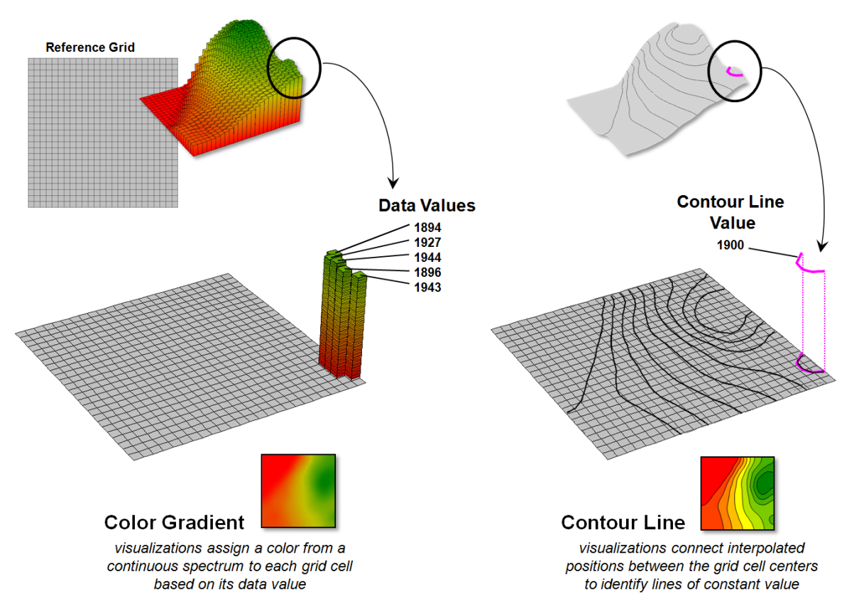
Figure 3. The x,y-coordinates
position surface information that can be displayed as continuously varying grid
cells of relative z-value heights (color gradient display) or as derived lines
of constant value (contour line display).
So what is the take-home from all this
discussion? First, surface data
(continuous) and contour lines (discontinuous) are not the same in either
theory or practice but are fundamentally different spatial expressions. A continuous color gradient is effective when
the underlying surface is a mathematical model or where the interval between
physical measurements is very small. In
these cases, the continuous color gradient is limited only by the resolution of
the display device.
Contour lines, on the other hand, are
effective to display coarse data. A
contour line display creates a series of lines at constant values that somewhat
“approximate” the gradient and provide the viewer with points of equal value
that serve as references for the changing surface.
For example, if a mountain region of Colorado
has elevation measurements taken every 100 feet, it would be impossible to
display the elevation of each individual square inch. In this scenario, a series of contour lines
describes the elevations in the region, with the understanding that the contour
lines are neither precise nor capture small bumps or depressions that occur
between the 100 foot measurements. If
more detailed measurements are taken, contour lines can be drawn closer
together, thus depicting greater detail of the underlying surface.
However, drawing contour lines close together
is ultimately limited both visually and computationally. When contour lines are too close together,
the lines themselves obscure the map, creating a useless blur. In addition, the processing time required to
compute and display a large number of contour lines renders the method
impractical.
This illustrates the beauty of the continuous
color gradient and contour line techniques—they are not same, hence they have
unique advantages and limitations that provide different data visualization
footholds for different spatial applications.
VtoR and Back!
(GeoWorld, December 2011)
The previous section described considerations
and procedures for deriving contour lines from map surfaces. The discussion emphasized the similarities and
differences between continuous/gradient map surfaces (raster) and
discontinuous/discrete spatial objects identifying points, lines and
polygons (vector).
Keep in mind that while raster treats
geographic space as a continuum, it can store the three basic types of discrete
map features—a point as a single grid cell, a line as a series of connecting
cells and a polygon as a set of contiguous cells. Similarly, vector can store generalizations
of continuous map surfaces as a series of contour lines or contour interval
polygons.
Paramount in raster data storage is the
concept of a data layer in which all of the categories have to be mutually
exclusive in space. That means that a
given grid cell in a Water map layer, for example, cannot be simultaneously classified
as a “spring” (e.g., category 1) and a “wetland” (e.g., category 2) at the same
unless an additional category is specified for the joint condition of “spring and
wetland” (e.g., category 12).
Another important consideration is that each
grid cell is assumed to be the same condition/characteristic throughout its
entirety. For example, a 30m grid cell
assigned as a spring does not infer a huge bubbling body of water in the shape
of a square— rather it denotes a cell location that contains a spring somewhere
within its interior. Similarly, a series
of stream cells does not imply a 30m wide flow of water that moves in a
saw-tooth fashion over the landscape— rather it identifies grid cells that
contain a stream somewhere within their interiors.
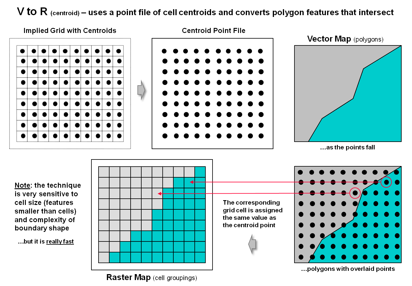
Figure 1. Basic procedure for
centroid-based vector to raster conversion (VtoR).
While raster data tends to generalize/lower
the spatial precision of map object placement and boundary, vector data
tends to generalize/lower the thematic accuracy of classification. For example, the subtle differences in a map
surface continuum of elevation have to be aggregated into broad contour interval
ranges to store the data as a discrete polygon.
Or, as in the case of contour lines, store a precise constant value but
impart no information for the space between the lines.
Hence the rallying cry of “VtoR
and back!” by grid-based GIS modelers echoes from the walls of cubicles
everywhere for converting between vector-based spatial objects and raster-based
grids. This enables them to access the
wealth of vector-based data, then utilize the thematic accuracy and analytical
power of continuous grid-based data and upon completion, push the model results
back to vector.
Figure 1 depicts the processing steps for a
frequently used method of converting vector polygons to contiguous groupings of
grid cells. It uses a point file of grid
centers and “point in polygon” processing to assign a value representing a
polygon’s characteristic/condition to every corresponding grid cell. In essence it is a statistical technique akin
to “dot grid” sampling that has been used in aerial photo interpretation and manual
map analysis for nearly 100 years. While
fast and straight forward for converting polygon data to cells, it is
unsuitable for point and line features.
In addition, if large cell-sizes are used, small polygons can be
missed.
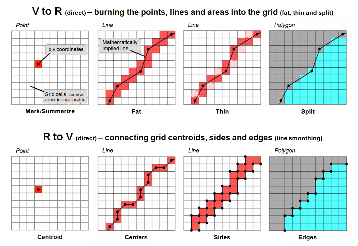
Figure 2. Basic procedures for
direct calculation-based vector to raster conversion (VtoR)
and the reverse (RtoV).
The top portion of figure 2 depicts an
alternative approach that directly “burns” the vector features into a grid
analogous to a branding iron or woodburning
tool. In the case of a point feature the
cell containing its x,y
coordinates is assigned a value representing the feature. The tricky part comes into play if there is
more than one point feature falling into a grid cell. Then the user must specify whether to simply
note “one or more” for a binary map or utilize a statistical procedure to
summarize the point values (e.g, #count, sum,
average, standard deviation, maximum, minimum, etc.).
For line features there are two primary
strategies for VtoR conversion— fat and thin. Fat identifies every grid cell that is cut by
a line segment, even if it is just a nick at the corner. Thin, on the other hand, identifies the
smallest possible set of adjoining cells to characterize a line feature. While the “thin” option produces pleasing
visualization of a line, it discards valuable information. For example, if the line feature was of a
stream, then water law rights/responsibilities are applicable to all of the
cells with a “stream running through it” regardless of whether it is through
the center or just in a corner.
The upper-right inset in figure 2 illustrates
the conversion of adjacent polygons. The
“fat” edges containing the polygon boundary are identified and geometry is used
to determine which polygon is mostly contained within each edge cell. All of the interior cells of a polygon are
identified to finish the polygon conversion.
On rare occasions the mixed cells containing boundary line are given a
composite number identifying the two characteristics/conditions. For example, if a soil map had two soil types
of 1 and 2 occurring in the same cell, the value 12 might be stored for the
boundary condition with 1 and 2 assigned to the respective interior cells. If the polygons are not abutting but
scattered across the landscape, the boundary cells (either fat or thin) are
assigned the same value as the interior cells with the exterior cells assigned
a background value.
The lower portion of figure 2 depicts approaches for converting raster to vector. For single cell locations, the x,y coordinates of a cell’s centroid is used to position a point feature and the cell value is used to populate the attribute table. On rare occasion where the cell value indicates the number of points contained in a cell, a random number generator is used to derive coordinates within the cell’s geographic extent for the set of points.
For gridded line features, the x,y coordinates of the of the centroids (thin) are frequently used to define the line segments. Often the set of points are condensed as appropriate and a smoothing equation applied to eliminate the saw-tooth jaggies. A radically different approach converts the sides of the cells into a thin polygon capturing the area of possible inclusion of the grid-based line— sort of a narrow corridor for the line.
For gridded polygons, the sides at the edges of abutting cells are used to define the feature’s boundary line and its points are condensed and smoothed with topology of the adjoining polygons added. For isolated gridded polygons, the outside edges are commonly used for identifying the polygon’s boundary line.
Figure 3 deals with converting continuous map surfaces to discrete vector representations. A frequently used technique that generates true contour lines of constant value was described in detail in the previous section. The procedure involves identifying cell values that bracket a desired contour level, then interpolating the x,y coordinates for points between all of the cell value pairs and connecting the new points for a line of constant value. The black lines in figure 3 identify the set interpolated 200 foot contour lines for a data set with values from 500 to 2500.
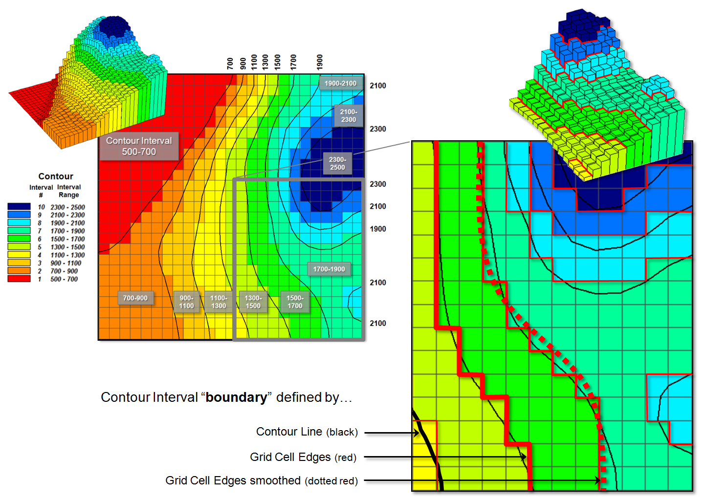
Figure 3. Comparison of the basic
approaches for identifying contour lines and contour interval boundaries.
Another commonly used technique involves
slicing the data range into a desired number of contour intervals. For example, 2500-500 / 10 = 200 identifies
the data step used in generating the data ranges of the contour intervals
(color bands) shown in the figure. The
first contour range from 500 to 700 “color-fills” with red all of the grid
cells having values that fall within this range; orange for values 700 to 900;
tan for values 900 to 1100; and so forth.
The 3D surface shows the contour interval classification draped over the
actual data values stored in the grid.
The added red lines in the enlarged inset
identify the edges of the grid cell contour interval groupings. As you can see in the enlarged 3D plot there
are numerous differing data values as the red border goes up and down with the
data values along the sawtooth edge. As previously noted this boundary can be
smoothed (dotted red) and used for the borders of the contour interval polygons
generated in the RtoV conversion.
The bottom line (pun intended) is that in many mapped data visualizations the boundary (border) outlining a contour interval is not the same as a contour line (line of constant value). That’s the beauty of grid vs. vector data structures— they are not the same, and therefore, provide for subtly and sometimes radically different perspectives of the patterns and relationships in spatial information—“V-tore and back!” is the rallying cry.
Setting a Place at the
Table for Grid-based Data
(GeoWorld, June 2013)
First the bad news—spatial data structure, formats and storage schemes tend to be a deep dive into a quagmire of minutia from which few return. The good news is that is the realm of vector data and this month’s journey is into the Land of Grids where things are quite regular and straight forward (for the most part).
At its conceptual foundation, grid-based map
data is simply a matrix of values with a specified number of rows and columns (configuration)
that is referenced to a specific location on the earth’s surface (geo-registered). It’s as if you tore out a spreadsheet and
stretched and tugged until its rectangular boxes
formed squares (grid cell) to cover a portion of the landscape. The value assigned to each grid summarizes
the characteristic or condition of a spatial variable (map layer) at
that location. Additional aligned
worksheets piled on top (map stack) describe other important
geographically-based variables—just a stack of numbers towering over a
continuous set of regularly-spaced grid cells (analysis frame) depicting
what occurs at every location throughout an area.
There are no differing types of map features,
irregular shapes, missing puzzle pieces, complex topology about neighboring
pieces, overlapping borders, serially linked files or other confounding
concepts to wade through. It is just a
set of organized grid cells containing information about every location. The only major difference in storage
approaches is whether the matrices are stored as individual “files” or as a
“table.”
Figure 1 depicts the data organization for Esri’s Grid ASCII export format as a single independent “file.” The first six records in the file identify
the geo-registration and configuration information (bottom left-side of the
figure). Note that the geo-registration
is identified in decimal degrees of latitude and longitude for the lower-left
corner of the matrix. The configuration
is identified as the number of columns and rows with a specified cell size that
defines the matrix. In addition a “no
data” value is set to indicate locations that will be excluded from
processing.
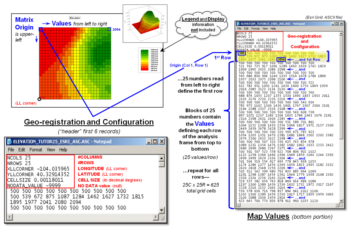
Figure 1. Storing grid maps as independent files is a
simple and flexible approach that has been used for years.
The remainder of the grid map file contains blocks
of values defining individual rows of the analysis frame that are read left to
right, top to the bottom, as you would read a book. In the example, each row is stored as a block
of 25 values that extends for 25 blocks for a total of 625 values. In a typical computer, the values are stored
as double-precision (64 bit) floating point numbers which provides a range of
approximately 10−308 to 10308 (really small to
really big numbers) capable of handling just about any map-ematical
equation.
Each grid map is stored as a separate file and
in the export format no legend or display information is provided. However in native ArcGIS grid format, this
ancillary information is carried and individual grid maps can be clipped,
adjusted and resized to form a consistent map stack for analysis stored as a
group of individual flat files.
Figure 2 illustrates the alternative “table”
format for storing grid-based mapped data.
In the table, each grid layer is stored as a separate column (field)
with their common grid cell locations identified as an informational line
(records). Each line in the table
identifies all of the spatial information for a given grid location in a
project area. In the example, strings of
25 values in a column define rows in the matrix read left to right. However in this example, the matrix origin
and the geo-registration origin align and the matrix rows are read from the
bottom row up to the top. The assignment
of the matrix origin is primarily a reflection of a software developer’s background—lower-left
for science types and upper-left for programmer types. Configuration information, such as 99.94 feet
for the cell size, is stored as header lines while the geo-registration of a
grid cell’s centroid can be explicitly stored as shown or implicitly inferred
by a map value’s position (line#) in the string of numbers. When map-ematical
analysis creates a new map its string of map values is added to the table as a
new column instead of being stored in an individual file.
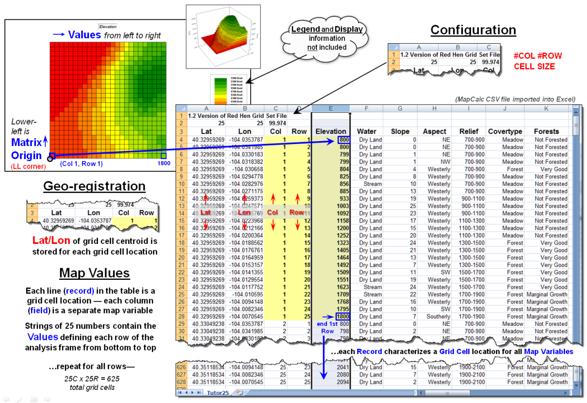
Figure 2.
Storing groups of commonly geo-referenced and configured grid maps in a table
provides consistency and uniformity that facilitates map analysis and modeling.
The relative advantages/disadvantages of the
file versus table approach to grid map storage have been part of the GIS
community debate for years. Most GIS
systems use independent files because of their legacy, simplicity and
flexibility. The geo-referencing and
configuration of the stored grid maps can take any form and “on-the-fly”
processing can be applied to account for the consistency needed in map
analysis.
However, with the increased influence of
remotely sensed data with inter-laced spectral bands and television with
interlaced signal processing, interest in the table approach has been on the
rise. In addition, relational database
capabilities have become much more powerful making “table maintenance” faster,
less problematic and more amenable to compression techniques.
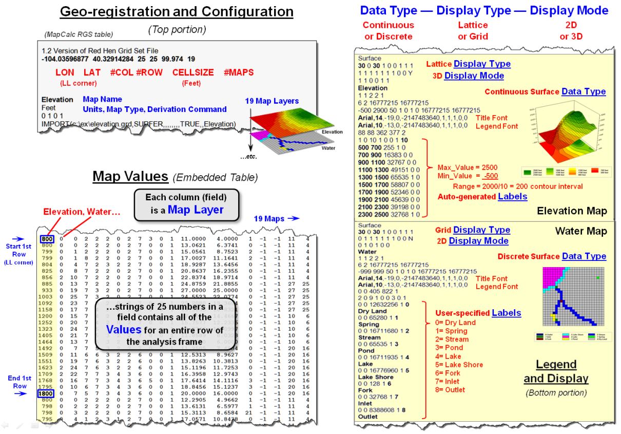
Figure 3. Combining all three basic elements for
storing grid maps (geo-registration/configuration, map values and
legend/display) sets the stage for fully optimized relation database tables for
the storage of grid-based data.
Figure 3 shows the organizational structure for
an early table-based system (MapCalc).
The top portion of the table identifies the common geo-registration and
configuration information shared by all of the map layers contained in the map
set. In the example, there are 19 map
layers listed whose values form an embedded table (bottom-left) as described in
figure 2.
The right-side of the figure depicts the
storage of additional legend and display information for two of the map
layers. The three display considerations
of Data Type (continuous or discrete), Display Type (lattice or
grid) and Display Mode (2D or 3D) are identified and specific graphics
settings, such as on/off grid mesh, plot cube appearance, viewing direction,
etc., are contained in the dense sets of parameter specifications.
Similarly, Legend Labeling and
associated parameters are stored, such as assigned color for each display
category/interval. When a map layer is
retrieved for viewing its display and legend parameters are read and the appropriate
graphical rendering of the map values in the matrix is produced. If a user changes a display, such as rotating
and tilting a 3D plot, the corresponding parameters are updated.
When a new map is created through map analysis
its map name, map type and derivation command is appended to the top portion of
the table; its map values are appended as a new field to the table in the
middle portion; and a temporary set of display and labeling parameters are
generated depending on the nature of the processing and the data type
generated. While all this seems
overwhelming to a human, the “mechanical” reading and writing to a structured,
self-documenting table is a piece-of-cake for a computer.
The MapCalc table format for grid-based data
was created in the early 1990s. While it
still serves small project areas very well (e.g., a few thousand acre farm or
research site), modern relational database techniques would greatly improve the
approach.
For the technically astute, the full dB design
would consist of three related tables: Map Definition Table containing
the MapID (“primary key” for joining tables) and
geo-registration/configuration information, a Grid Layer Definitions Table
containing the MapID, LayerID
and legend/display information about the data layer, and a third Cell
Definition Table containing MapID/LayerID plus all of the map values in the matrix organized
by the primary key of MapID à RowNumber à ColumnNumber.
Organizing the three basic elements for
storing grid maps (geo-registration/configuration, map values and
legend/display) into a set of linked tables and structuring the relationships
between tables is a big part of the probable future of grid-based map analysis
and modeling. Also, it sets the stage
for a follow-on argument supporting the contention that latitude/longitude
referencing of grid-based data is the “universal spatial database key” (spatial
stamp) that promises to join disparate data sets in much the same way as the
date/time stamp—sort of the Rosetta Stone of geotechnology.
_____________________________